没有合适的资源?快使用搜索试试~ 我知道了~
brady -rock mechanics 4
需积分: 0 2 下载量 41 浏览量
2011-04-29
11:18:48
上传
评论
收藏 1.87MB PDF 举报
温馨提示
试读
57页
The engineering mechanics-based approach to the solution of mining rock mechanics problems used in this book, requires prior definition of the stress–strain behaviour of the rock mass. Important aspects of this behaviour are the constants relating stresses and strains in the elastic range, the stress levels at which yield, fracturing or slip occurs within the rock mass, and the post-peak stress–strain behaviour of the fractured or ‘failed’ rock.
资源详情
资源评论
资源推荐
4
Rock strength and deformability
4.1 Introduction
The engineering mechanics-based approach to the solution of mining rock mechanics
problems used in this book, requires prior definition of the stress–strain behaviour of
the rock mass. Important aspects of this behaviour are the constants relating stresses
and strains in the elastic range, the stress levels at which yield, fracturing or slip occurs
within the rock mass, and the post-peak stress–strain behaviour of the fractured or
‘failed’ rock.
In some problems, it may be the behaviour of the intact rock material that is of
concern. This will be the case when considering the excavation of rock by drilling
and blasting, or when considering the stability of excavations in good quality, brittle
rock which is subject to rockburst conditions. In other instances, the behaviour of
single discontinuities,orofasmall number of discontinuities, will be of paramount
importance. Examples of this class of problem include the equilibrium of blocks of
rock formed by the intersections ofthree or morediscontinuities and the roof or wall of
an excavation, and cases in which slip on a major throughgoing fault must be analysed.
A different class of problem is that in which the rock mass must be considered as
an assembly of discrete blocks.Asnoted in section 6.7 which describes the distinct
element method of numerical analysis, the normal and shear force–displacement
relations at block face-to-face and corner-to-face contacts are of central importance
in this case. Finally, it is sometimes necessary to consider the global response of a
jointed rock mass in which the discontinuity spacing is small on the scale of the
problem domain. The behaviour of caving masses of rock is an obvious example of
this class of problem.
It is important to note that the presence of major discontinuities or of a number of
joint sets does not necessarily imply that the rock mass will behave as a discontinuum.
In mining settings in which the rock surrounding the excavations is always subject
to high compressive stresses, it may be reasonable to treat a jointed rock mass as an
equivalent elastic continuum. A simple example of the way in which rock material
and discontinuity properties may be combined to obtain the elastic properties of the
equivalent continuum is given in section 4.9.2.
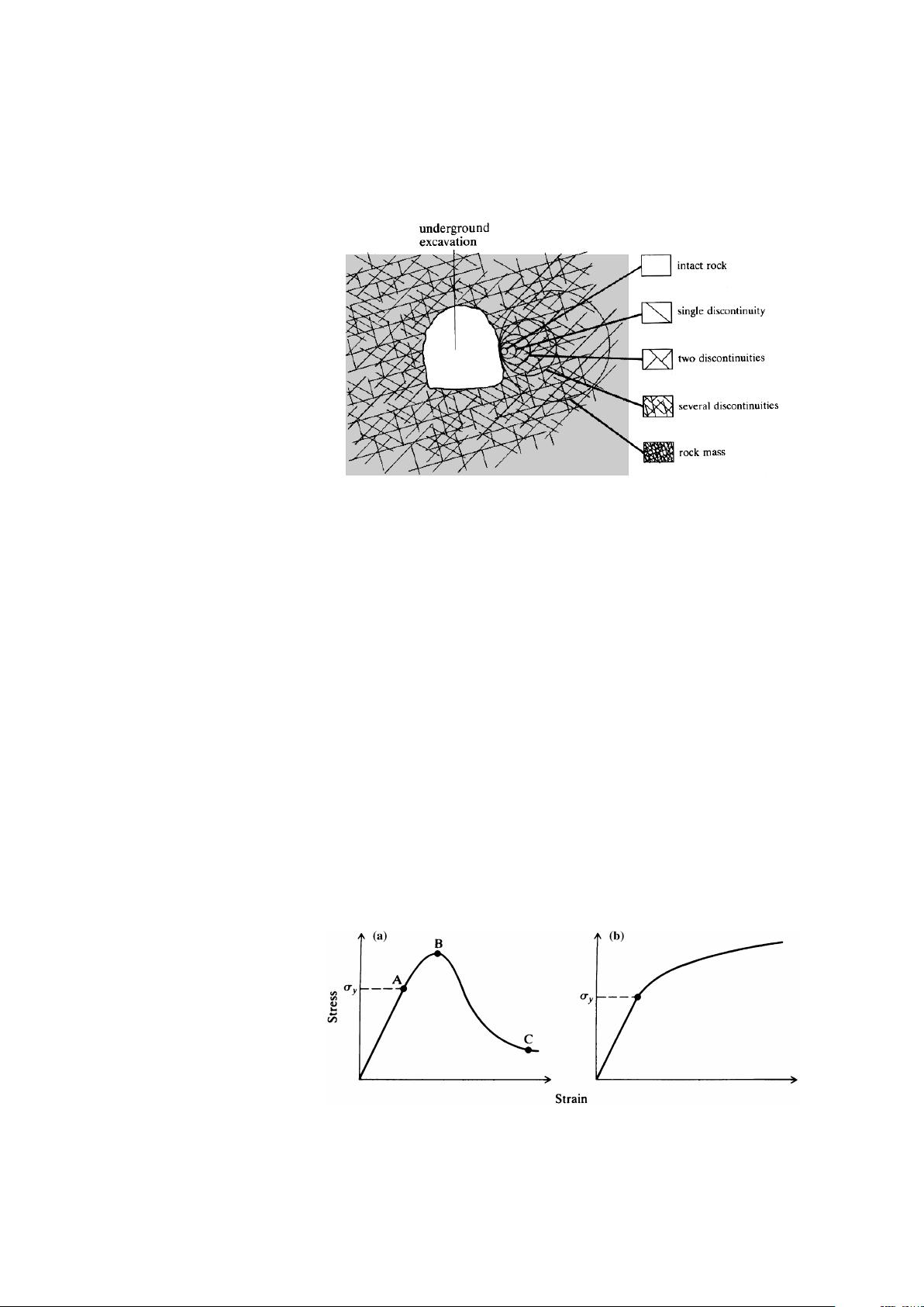
Figure 4.1 illustrates the transition from intact rock to a heavily jointed rock mass
with increasing sample size in a hypothetical rock mass surrounding an underground
excavation. Which model will apply in a given case will depend on the size of the
excavation relative to the discontinuity spacing, the imposed stress level, and the
orientations and strengths of the discontinuities. Those aspects of the stress–strain
behaviour of rocks and rock masses required to solve these various classes of prob-
lem, will be discussed in this chapter. Since compressive stresses predominate in
geotechnical problems, the emphasis will be on response to compressive and shear
stresses. For the reasons outlined in section 1.2.3, the response to tensile stresses will
not be considered in detail.
85
ROCK STRENGTH AND DEFORMABILITY
Figure 4.1 Idealised illustration of
the transition from intact rock to a
heavily jointed rock mass with in-
creasing sample size (after Hoek and
Brown, 1980).
4.2 Concepts and definitions
Experience has shown that the terminology used in discussions of rock ‘strength’ and
‘failure’ can cause confusion. Unfortunately, terms which have precise meanings in
engineering science are often used imprecisely in engineering practice. In this text,
the following terminology and meanings will be used.
Fracture is the formation of planes of separation in the rock material. It involves
the breaking of bonds to form new surfaces. The onset of fracture is not necessarily
synonymous with failure or with the attainment of peak strength.
Strength,orpeak strength,isthe maximum stress, usually averaged over a plane,
that the rock can sustain under a given set of conditions. It corresponds to point B
in Figure 4.2a. After its peak strength has been exceeded, the specimen may still
have some load-carrying capacity or strength. The minimum or residual strength
is reached generally only after considerable post-peak deformation (point C in
Figure 4.2a).
Brittle fracture is the process by which sudden loss of strength occurs across a
plane following little or no permanent (plastic) deformation. It is usually associated
with strain-softening or strain-weakening behaviour of the specimen as illustrated in
Figure 4.2a.
Ductile deformation occurs when the rock can sustain further permanent defor-
mation without losing load-carrying capacity (Figure 4.2b).
Figure 4.2 (a) Strain-softening; (b)
strain-hardening stress–strain curves.
86
BEHAVIOUR OF ISOTROPIC ROCK MATERIAL IN UNIAXIAL COMPRESSION
Yield occurs when there is a departure from elastic behaviour, i.e. when some of
the deformation becomes irrecoverable as at A in Figure 4.2a. The yield stress (
y
in
Figure 4.2) is the stress at which permanent deformation first appears.
Failure is often said to occur at the peak strength or be initiated at the peak strength
(Jaeger and Cook, 1979). An alternative engineering approach is to say that the rock
has failed when itcan no longer adequately support the forces applied to it or otherwise
fulfil its engineering function. This may involve considerations of factors other than
peak strength. In some cases, excessive deformation may be a more appropriate
criterion of ‘failure’ in this sense.
Effective stress is defined, in general terms, as the stress which governs the gross
mechanical response of a porous material. The effective stress is a function of the
total or applied stress and the pressure of the fluid in the pores of the material,
known as the pore pressure or pore-water pressure. The concept of effective stress
was first developed by Karl Terzaghi who used it to provide a rational basis for the
understanding of the engineering behaviour of soils. Terzaghi’s formulation of the
law of effective stress,anaccount of which is given by Skempton (1960), is probably
the single most important contribution ever made to the development of geotechnical
engineering. For soils and some rocks loaded under particular conditions, the effective
stresses,
ij
, are given by
ij
=
ij
− u
ij
(4.1)
where
ij
are the total stresses, u is the pore pressure, and
ij
is the Kronecker delta.
This result is so well established for soils that it is often taken to be the definition of
effective stress. Experimental evidence and theoretical argument suggest that, over a
wide range of material properties and test conditions, the response of rock depends
on
ij
=
ij
− u
ij
(4.2)
where
1, and is a constant for a given case (Paterson, 1978).
4.3 Behaviour of isotropic rock material in uniaxial compression
4.3.1 Influence of rock type and condition
Uniaxial compression of cylindrical specimens prepared from drill core, is proba-
bly the most widely performed test on rock. It is used to determine the uniaxial or
unconfined compressive strength,
c
, and the elastic constants, Young’s modulus,
E, and Poisson’s ratio, ,ofthe rock material. The uniaxial compressive strength
of the intact rock is used in rock mass classification schemes (section 3.7), and as
a basic parameter in the rock mass strength criterion to be introduced later in this
chapter.
Despite its apparent simplicity, great care must be exercised in interpreting results
obtained in the test. Obviously, the observed response will depend on the nature and
composition of the rock and on the condition of the test specimens. For similar miner-
alogy,
c
will decrease with increasing porosity, increasing degree of weathering and
increasing degree of microfissuring. As noted in section 1.2.4,
c
may also decrease
87
ROCK STRENGTH AND DEFORMABILITY
with increasing water content. Data illustrating these various effects are presented by
Vutukuri et al. (1974).
It must be recognised that, because of these effects, the uniaxial compressive
strengths of samples of rock having the same geological name, can vary widely.
Thus the uniaxial compressive strength of sandstone will vary with the grain size,
the packing density, the nature and extent of cementing between the grains, and the
levels of pressure and temperature that the rock has been subjected to throughout
its history. However, the geological name of the rock type can give some qualitative
indication of its mechanical behaviour. For example, a slate can be expected to exhibit
cleavage which will produce anisotropic behaviour, and a quartzite will generally be a
strong, brittle rock. Despite the fact that such features are typical of some rock types,
it is dangerous to attempt to assign mechanical properties to rock from a particular
location on the basis of its geological description alone. There is no substitute for a
well-planned and executed programme of testing.
4.3.2 Standard test procedure and interpretation
Suggested techniques for determining the uniaxial compressive strength and deforma-
bility of rock material are given by the International Society for Rock Mechanics
Commission on Standardization of Laboratory and Field Tests (ISRM Commission,
1979). The essential features of the recommended procedure are:
(a) The test specimens should be right circular cylinders having a height to diam-
eter ratio of 2.5–3.0 and a diameter preferably of not less than NX core size,
approximately 54 mm. The specimen diameter should be at least 10 times the
size of the largest grain in the rock.
(b) The ends of the specimen should be flat to within 0.02 mm and should not depart
from perpendicularity to the axis of the specimen by more than 0.001 rad or
0.05 mm in 50 mm.
(c) The use of capping materials or end surface treatments other than machining is
not permitted.
(d) Specimens should be stored, for no longer than 30 days, in such a way as to
preserve the natural water content, as far as possible, and tested in that condition.
(e) Load should be applied to the specimen at a constant stress rate of
0.5–1.0MPas
−1
.
(f ) Axial load and axial and radial or circumferential strains or deformations should
be recorded throughout each test.
(g) There should be at least five replications of each test.
Figure 4.3 shows an example of the results obtained in such a test. The axial force
recorded throughout the test has been divided by the initial cross-sectional area of
the specimen to give the average axial stress,
a
, which is shown plotted against
overall axial strain, ε
a
, and against radial strain, ε
r
. Where post-peak deformations
are recorded (section 4.3.7), the cross-sectional area may change considerably as
the specimen progressively breaks up. In this case, it is preferable to present the
experimental data as force–displacement curves.
In terms of progressive fracture development and the accumulation of deformation,
the stress-strain or load-deformation responses of rock material in uniaxial compres-
sion generally exhibit the four stages illustrated in Figure 4.3. An initial bedding down
and crack closure stage is followed by a stage of elastic deformation until an axial
88
BEHAVIOUR OF ISOTROPIC ROCK MATERIAL IN UNIAXIAL COMPRESSION
Figure4.3 Resultsobtained ina uni-
axial compression test on rock.
stress of
ci
is reached at which stable crack propagation is initiated. This continues
until the axial stress reaches
cd
when unstable crack growth and irrecoverable defor-
mations begin. This region continues until the peak or uniaxial compressive strength,
c
,isreached. The processes involved in these stages of loading will be discussed
later in this Chapter.
As shown in Figure 4.3, the axial Young’s modulus of the specimen varies through-
out the loading history and so is not a uniquely determined constant for the material.
It may be calculated in a number of ways, the most common being:
(a) Tangent Young’s modulus, E
t
,isthe slope of the axial stress–axial strain curve
at some fixed percentage, generally 50%, of the peak strength. For the example
shown in Figure 4.3, E
t
= 51.0GPa.
(b) Average Young’s modulus, E
av
,isthe average slope of the more-or-less straight
line portion of the axial stress–strain curve. For the example shown in Figure
4.3, E
av
= 51.0GPa.
(c) Secant Young’s modulus, E
s
,isthe slope of a straight line joining the origin
of the axial stress–strain curve to a point on the curve at some fixed percentage
of the peak strength. In Figure 4.3, the secant modulus at peak strength is E
s
=
32.1GPa.
Corresponding to any value of Young’s modulus, a value of Poisson’s ratio may be
calculated as
=−
(
a
/ε
a
)
(
a
/ε
r
)
(4.3)
For the data given in Figure 4.3, the values of corresponding to the values of E
t
,
E
av
, and E
s
calculated above are approximately 0.29, 0.31 and 0.40 respectively.
Because of the axial symmetry of the specimen, the volumetric strain, ε
v
,atany
stage of the test can be calculated as
ε
v
= ε
a
+ 2ε
r
(4.4)
Forexample, at a stress level of
a
= 80 MPa in Figure 4.3, ε
a
= 0.220%, ε
r
=
−0.055% and ε
v
= 0.110%.
89
剩余56页未读,继续阅读
nie_wen
- 粉丝: 1
- 资源: 2
上传资源 快速赚钱
- 我的内容管理 展开
- 我的资源 快来上传第一个资源
- 我的收益 登录查看自己的收益
- 我的积分 登录查看自己的积分
- 我的C币 登录后查看C币余额
- 我的收藏
- 我的下载
- 下载帮助
安全验证
文档复制为VIP权益,开通VIP直接复制
信息提交成功
评论0