YOLO-CIANNA：在无线电数据中进行深度学习的星系检测I.一种受YOLO启发的新型源检测方法应用于SKAOSDC1资源-CSDN文库

版权申诉

200 浏览量 2024-04-11 15:16:16 上传评论收藏 4.27MB PDF 举报

资源推荐

资源详情

资源评论

Astronomy & Astrophysics manuscript no. yolo_sdc1_paper ©ESO 2024

February 9, 2024

YOLO-CIANNA: Galaxy detection with deep learning in radio data

I. A new YOLO-inspired source detection method applied to the SKAO SDC1

D. Cornu

, P. Salomé

, B. Semelin

, A. Marchal

2, 3

, J. Freundlich

, S. Aicardi

X. Lu

, G. Sainton

, F. Mertens

, F. Combes

1, 7

, C. Tasse

8, 9

LERMA, Observatoire de Paris, PSL research Université, CNRS, Sorbonne Université, 75014, Paris, France

Canadian Institute for Theoretical Astrophysics, University of Toronto, 60 St. George Street, Toronto, ON M5S 3H8

Research School of Astronomy & Astrophysics, Australian National University, Canberra ACT 2610 Australia

Université de Strasbourg, CNRS UMR 7550, Observatoire astronomique de Strasbourg, 67000 Strasbourg, France

DIO, Observatoire de Paris, CNRS, PSL, 75014, Paris, France

IDRIS, CNRS, F-91403 Orsay, France

Collège de France, 11 Place Marcelin Berthelot, 75005, Paris, France

GEPI, Observatoire de Paris, CNRS, Université Paris Diderot, 5 Place Jules Janssen, 92190, Meudon, France

Department of Physics & Electronics, Rhodes University, PO Box 94, Grahamstown, 6140, South Africa

Received ..., ...; accepted ..., ...

ABSTRACT

Context. The upcoming Square Kilometer Array (SKA) will set a new standard regarding data volume generated by an astronomical

instrument, which is likely to challenge widely adopted data analysis tools that scale inadequately with the data size.

Aims. This study aims to develop a new source detection and characterization method for massive radio astronomical datasets by

adapting modern deep-learning object detection techniques. These approaches have proved their eﬃciency on complex computer

vision tasks, and we seek to identify their speciﬁc strengths and weaknesses when applied to astronomical data.

Methods. We introduce YOLO-CIANNA, a highly customized deep-learning object detector designed speciﬁcally for astronomical

datasets. This paper presents the method and describes all the low-level adaptations required to address the speciﬁc challenges of radio-

astronomical images. We demonstrate this method’s capabilities using simulated 2D continuum images from the SKA Observatory

(SKAO) Science Data Challenge 1 (SDC1) dataset.

Results. Our method outperforms every other published result on the speciﬁc SDC1 dataset. Using the SDC1 metric, we improve the

challenge-winning score by +139% and the score of the only other post-challenge participation by +61%. Our catalog has a detection

purity of 94% while detecting 40 to 60 % more sources than previous top-score results with a total of almost 680000 properly detected

sources. The trained model can also be forced to reach 99% purity in post-process and still detect 10 to 30% more sources than the

other top-score methods. Our method is eﬃcient at low signal-to-noise ratio and exhibits strong characterization accuracy. It is also

capable of real-time detection, with a peak prediction speed of 500 images of 512×512 pixels per second on a single GPU.

Conclusions. YOLO-CIANNA achieves state-of-the-art detection and characterization results on the simulated SDC1 dataset. This is

encouraging regarding its potential capability over observational data from SKA precursors. The method is open source and included

in the wider CIANNA framework. We provide scripts to train and apply this method to the SDC1 dataset in the CIANNA repository.

Key words. Methods: numerical – Methods: statistical – Methods: data analysis – Galaxies: statistics – Radio continuum: galaxies

1. Introduction

Modern astronomical instruments generate ever-increasing data

volumes, following the need for better resolution, sensitivity,

and larger wavelength coverage. Astronomical datasets are often

highly dimensional and require precise encoding of the measure-

ments due to a high dynamic range. In addition, it is often nec-

essary to preserve the raw data due to iterative improvement of

the analysis pipelines. Radio-astronomy is strongly aﬀected by

the explosion of data volumes, especially regarding giant radio

interferometers. In particular, the upcoming Square Kilometer

Array (SKA, Braun et al. 2019) is expected to have an unprece-

dented real-time data rate and to produce a remarkable amount

of stored science data products with around 700 PB of archived

data per year. This instrument is foreseen to have the necessary

sensitivity to set constraints on the cosmic dawn and the epoch

of reionization and to trace the evolution of astronomical objects

over cosmological times. With such volume and complexity of

data, some classical analysis methods and tools employed in ra-

dio astronomy for decades start to exhibit scaling limits.

In this context, the SKA Observatory (SKAO) started the

organization of recurrent Science Data Challenges (SDCs) to

gather astronomers from the international community around

simulated datasets that resemble future SKA data products. The

objective is to evaluate the suitability of existing analysis meth-

ods and encourage the development of new ones. It is also an

opportunity for astronomers to get familiar with the nature of

such datasets and to gain experience in their exploration.

The ﬁrst edition, SDC1 (Bonaldi et al. 2021), focused on a

source detection and characterization task over simulated contin-

uum radio images at diﬀerent frequencies and integration times.

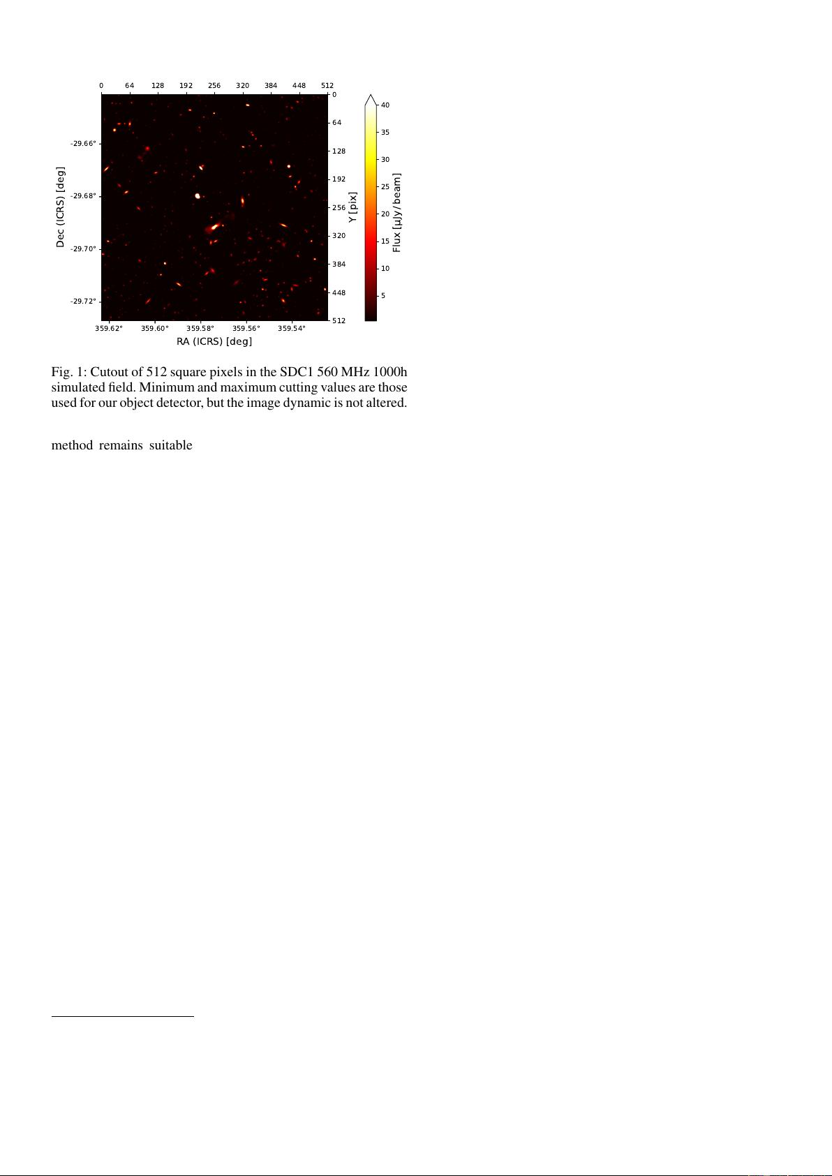
We show a cutout from one of the SDC1 images in Fig. 1, illus-

trating the source density and the high dynamical range. Source-

Article number, page 1 of 40

arXiv:2402.05925v1 [astro-ph.IM] 8 Feb 2024

A&A proofs: manuscript no. yolo_sdc1_paper

ﬁnding is a common task in astronomy and is often the ﬁrst anal-

ysis to be done on a newly acquired image product. It is already

performed by a variety of classical methods, for example, SEx-

tractor (Bertin & Arnouts 1996), SFIND (Hopkins et al. 2002),

CUTEX (Molinari et al. 2011), BLOBCAT (Hales et al. 2012),

AEGEAN (Hancock et al. 2018), DUCHAMP (Whiting 2012),

PyBDSF (Mohan & Raﬀerty 2015), PROFOUND (Robotham

et al. 2018). The obtained source catalogs can then be augmented

with characterization information and used as primary data for

subsequent analyses. This task is strongly aﬀected by the in-

crease in volume and dimensionality, making it a good proxy

to evaluate the upcoming data handling challenges.

In the past decade, we observed an explosion in the machine

learning (ML) methods usage in all ﬁelds, including astronomy

and astrophysics (Huertas-Company & Lanusse 2023). One of

the advantages of ML methods is their good performance and

eﬃciency scaling with data size and dimensionality. There is a

considerable variety of ML approaches, so we only focus here on

methods based on the deep artiﬁcial neural networks formalism

(LeCun et al. 2015). Deep learning approaches have been ex-

tensively used for computer vision tasks, including the leading

object detection application (Russakovsky et al. 2015; Evering-

ham et al. 2010; Lin et al. 2014). While detection models have

been extensively used in other domains for several years, they

are not yet widely adopted in the astronomical community.

Deep learning object detection methods are usually sepa-

rated into three families (Zhao et al. 2018). The ﬁrst one repre-

sents segmentation models. Their main advantage is identifying

which pixels belong to a given object type (semantic segmenta-

tion). Their main drawback is their symmetric structure (encoder

and decoder) and the amount of work to be done near the image

resolution, making them compute-intensive. They can also be

used as a convenient structure for denoising tasks. This family

is mainly represented by the U-Net (Ronneberger et al. 2015)

method. Due to their proximity with classical source detection

approaches, they have been employed for a variety of astronom-

ical applications (e.g., Akeret et al. 2017; Vafaei Sadr et al. 2019;

Lukic et al. 2019; Paillassa et al. 2020; Bianco et al. 2021; Maki-

nen et al. 2021; Sortino et al. 2023; Håkansson et al. 2023).

The second family corresponds to the region-based detectors.

They are often based on multi-stage neural networks that split the

detection task into a region proposal step and a detection reﬁne-

ment step. They are the most employed for mission-critical tasks

due to their accuracy. While faster than segmentation methods,

the high detection accuracy models are compute-intensive due

to the multi-stage process. This family is mainly represented by

the R-CNN method (Girshick et al. 2013) and all its derivatives

(e.g., Fast R-CNN, Faster R-CNN). Examples of astronomical

applications with these methods are more limited, but it is in-

creasing (e.g., Wu et al. 2019; Jia et al. 2020; Lao et al. 2021; Yu

et al. 2022; Sortino et al. 2023). There is a special variation of

these methods that combines the region-based detection formal-

ism with a mask prediction used to perform instance segmenta-

tion. They are mainly represented by the Mask R-CNN method

(He et al. 2017), which is also increasingly used in astronomy

(e.g., Burke et al. 2019; Farias et al. 2020; Riggi et al. 2023;

Sortino et al. 2023). We note that region-based methods are com-

monly combined with feature pyramid network (Lin et al. 2016),

which helps represent multiple scales in the detection task.

The last family consists of regression-based detectors, which

are mostly based on single-stage neural networks. These meth-

ods are compute-eﬃcient and often used for real-time object de-

tection. They are mainly represented by the YOLO method and

its sub-versions (Redmon et al. 2015; Redmon & Farhadi 2016,

2018), but we can also cite SSD (Liu et al. 2015). There have

been a few astronomical applications, mostly in the visible do-

main (González et al. 2018; He et al. 2021; Wang et al. 2021;

Grishin et al. 2023; Xing et al. 2023).

We highlight that methods based on transformers (Vaswani

et al. 2017) are now common in computer vision (Carion et al.

2020), and astronomical applications are just starting to be pub-

lished (Gupta et al. 2024; He et al. 2023). We also note that some

methods include deep learning parts in more classical source

detection tools, which can improve the detection purity or the

source characterization (e.g., Tolley et al. 2022). More refer-

ences regarding deep learning methods for source detection can

be found in Sortino et al. (2023) an Ndung’u et al. (2023).

This is the ﬁrst paper of a series that aims to present a

new source detection and characterization method called YOLO-

CIANNA that was developed and used in the context of MIN-

ERVA’s (MachINe lEarning for Radioastronomy at Observatoire

de Paris) team participation in the SDC2 (Hartley et al. 2023),

enabling it to achieve ﬁrst place. This ﬁrst paper describes the

method and presents its application over simulated 2D contin-

uum images from the SDC1 dataset. A second paper will present

an application over simulated 3D cubes of HI emission using the

SDC2 dataset. The series will then continue applying the method

to observational data from several SKA precursors.

The primary objective of this ﬁrst paper is to describe the

YOLO-CIANNA method, which is done in Sect. 2, and to

present how we adapted it to account for the speciﬁc challenges

of astronomical source detection. In Sect. 3, we present the

SDC1 dataset, composed of comprehensive 2D images, and ex-

pose how we used it to construct a benchmark to evaluate our

method’s detection and characterization capabilities. In Sect. 4,

we present the detection result of our method and do a detailed

analysis of the source catalog we obtained over the SDC1. We

use these results to highlight the strengths and weaknesses of

our detector, which are then discussed in Sect. 5. We also added

three signiﬁcant Appendix sections. The ﬁrst one, Appendix A,

presents the diﬀerences between our YOLO-CIANNA method

and the classical YOLO implementation. In Appendix B, we

present how the classical network architecture associated with

YOLO would perform on the SDC1. And ﬁnally, Appendix A,

presents an alternative training area deﬁnition for the SDC1.

2. Method

Our method was inspired by the You Only Look Once (YOLO,

Redmon et al. 2015; Redmon & Farhadi 2016, 2018) approach,

a regression-based deep learning object detector. While region-

based approaches like R-CNN (Girshick et al. 2013) are often

considered the most accurate object detectors, regression-based

methods present a straightforward single network architecture,

making them more compute-eﬃcient at a given detection accu-

racy. Both families can reach state-of-the-art accuracy depending

on implementation details and architecture design. YOLO-like

methods are usually preferred for real-time detection applica-

tions. In this context, our choice of exploring a YOLO-inspired

regression-based approach was driven by i) fewer implementa-

tion constraints, ii) a strong emphasis on compute performance

considering the upcoming data volume of radio-astronomical

surveys, and iii) the single network regression-based structure

on which it is easier to add more predictive capabilities.

In this section, we present the main design and properties

of our custom object detection method along with necessary

general concepts about object detection for non-expert read-

ers. Despite being depicted for an astronomical application, our

Article number, page 2 of 40

Cornu et al.: YOLO-CIANNA: Galaxy detection with deep learning in radio data

359.62° 359.60° 359.58° 359.56° 359.54°

-29.66°

-29.68°

-29.70°

-29.72°

RA (ICRS) [deg]

Dec (ICRS) [deg]

0 64 128 192 256 320 384 448 512

128

192

256

320

384

448

512

Y [pix]

Flux [ Jy/ beam]

Fig. 1: Cutout of 512 square pixels in the SDC1 560 MHz 1000h

simulated ﬁeld. Minimum and maximum cutting values are those

used for our object detector, but the image dynamic is not altered.

method remains suitable for general-purpose object detection

(Appendix A.8). For clarity, we describe the whole method from

scratch, which includes aspects from the classical YOLO im-

plementation and our dedicated modiﬁcations. The added or

modiﬁed elements in comparison to the three ﬁrst classical ver-

sions from the original author, YOLO-V1 (Redmon et al. 2015),

YOLO-V2 (Redmon & Farhadi 2016), and YOLO-V3 (Redmon

& Farhadi 2018) will be mentioned. Still, the more technical

and in-depth justiﬁcations for these changes are presented in

Appendix A. Even though the modiﬁcations we brought to the

YOLO algorithm are substantial, we still refer to our approach

as YOLO-CIANNA in this paper for the sake of simplicity.

The implementation was made inside the custom high-

performance deep learning framework CIANNA

(Convolu-

tional Interactive Artiﬁcial Neural Networks by/for Astrophysi-

cists). The implementation and usage details can be found on

the CIANNA wiki pages. For reproducibility purposes, we pro-

vide example scripts for training and applying the method to the

SDC1 dataset in the CIANNA git repository.

To ease the understanding of the technical parts of the paper

for readers unfamiliar with ML terminology, we list a few tech-

nical terms we use and the associated descriptions we have for

them. The most common ML terms are not deﬁned but can be

found in any proper ML textbook or review (LeCun et al. 2015).

– Bounding box: in classical computer vision, the smallest

rectangular box that includes all the visible pixels belonging

to a speciﬁc object in a given image.

– Expressivity: refers to the predictive strength of a network.

The higher the expressivity, the more complex or diverse the

predictions can be. The expressivity increases with the num-

ber of weights and layers in a network.

– Receptive ﬁeld: corresponds to all the input pixels that can

contribute to the activation of a neuron at a speciﬁc point in

the network. It represents the maximum size of the patterns

that can be identiﬁed in the input space.

– Reduction factor: the ratio between the input layer spatial

dimension and the output layer spatial dimension.

CIANNA is open source and freely accessible through GitHub

https://github.com/Deyht/CIANNA. The version used in this paper cor-

responds to the 1.0 release. DOI:xx.xxxx/xxxxx.xxxxxxx

2.1. Bounding boxes for object detection

Our method uses a fully convolutional neural network (CNN)

structure to construct a mapping from a 2D input image to a reg-

ular output grid of detection units. Each output grid cell repre-

sents a small area of the input image with a size that depends on

the ratio between the input and the output grid resolutions. Each

grid cell is tasked to detect all possible objects whose center is

located inside the input region it represents. To characterize an

object, we rely on the bounding box formalism that encodes an

object as a four-dimension vector composed of the box center

and its size (x, y, w, h), which are the quantities that the detection

units must predict. Our method belongs to the supervised learn-

ing approaches, so it relies on a training set composed of images

with a list of all the visible objects to be detected. Each object

can be encoded as a target bounding box that the detector will be

tasked to predict using only information from the input image.

This can be done through an optimization process, also called

learning, which is an iterative process that aims at minimizing a

loss function L, also called an error function, that compares the

target boxes with the predicted boxes at the current step. This

loss should encompass all the object properties to be predicted.

To ease the method description, we ﬁrst write an abstract loss as

L = L

pos

+ L

size

+ L

prob

+ L

ob j

+ L

class

+ L

param

. (1)

The aim of the Sects. 2.1 to 2.4 is to describe all of the loss

sub-parts. Our complete detailed loss function is presented in

Sect. 2.7 with Eq. 14.

For now, we only describe the case of a single box predic-

tion per grid cell. The more realistic case of multiple objects per

grid cell is presented in Sect. 2.5. To represent a bounding box,

each grid cell must predict a 4-element vector (o

, o

) that

maps to the box’s geometric properties following

x = o

+ g

, (2)

y = o

+ g

, (3)

w = p

)

, (4)

h = p

)

. (5)

Each grid cell is only tasked to position the object center

inside its dedicated area, which is obtained using two sigmoid-

activated values (o

, o

). The position of the grid cell in the full

image must then be added to obtain the real position of the ob-

ject, which is expressed by the (g

, g

) coordinates. The object

size is obtained by an exponential transform of the predicted

values (o

, o

) that acts as a scaling on a pre-deﬁned size prior

, p

). This is equivalent to an anchor-box formalism (Ren

et al. 2015) as discussed in Sect. 2.5. The corresponding bound-

ing box construction on the output grid is illustrated in Fig. 2.

With this formalism, it is possible to construct a network out-

put layer with a

⟨

, g

, 4

⟩

grid that is capable of positioning and

scaling a bounding box for each grid cell. For each prediction-

target pair, we use a sum-of-square error to compute the out-

put loss function for center coordinates and sizes (Sect. 2.7).

The error is not computed on the sigmoid-activated positions

but on the raw output for the sizes after target conversion using

ˆo

= log(w/p

) and ˆo

= log(h/p

). This results in the follow-

ing loss terms

pos

i=0

match



− ˆo

)

+ (o

− ˆo

)



, (6)

size

i=0

match



− ˆo

)

+ (o

− ˆo

)



, (7)

Article number, page 3 of 40

A&A proofs: manuscript no. yolo_sdc1_paper

Fig. 2: Illustration of the YOLO bounding box representation.

The diﬀerent quantities correspond to Eqs. 2 to 5. The dashed

black box corresponds to the theoretical prior (o

= o

= 0),

while the red box represents the scaled network predicted size.

where the hat values represent the target for the corresponding

predicted value, the sum over i represents all the grid cells with

= g

×g

, and 1

match

is a mask to identify the predicted boxes

that have an associated target box (Sect. 2.6). The grid cells

that do not contain any object have no contribution to these loss

terms. All these elements follow the classical YOLO formalism.

We discuss the possible limitations of using bounding boxes to

describe astronomical objects in Sect. 5.2.2.

We emphasize that nothing prevents the size of the predicted

box from being larger than the area mapped by a grid cell up

to the size of the full image. Each grid cell receives informa-

tion from a large area corresponding to the backbone network

receptive ﬁeld. The receptive ﬁelds of nearby grid cells usually

overlap, but a target box center can only lie in one grid cell.

Due to the fully convolutional structure required for our method,

each grid cell represents a localized prediction using identical

weights. It is equivalent to having a single detector that scans

diﬀerent regions of the same image but in a more eﬃcient way

from a network architecture standpoint. This approach is equiva-

lent to what is done starting with YOLO-V2 but diﬀers from the

one introduced in YOLO-V1. More details about the eﬀect of

the fully convolutional architecture and the corresponding out-

put grid encoding are provided in Appendix A.1 and A.2.

2.2. Detection probability and objectness score

To obtain a working object detector, we not only have to pre-

dict bounding boxes but also to evaluate the chances that they

indeed contain an object. For this, we add a self-assessed de-

tection probability prediction P to each detection unit, which is

constrained during training. This term uses a sigmoid activation

and adds a sum-of-square error contribution to the loss. Due to

our grid structure, we have one possible box per grid cell. In a

context with only a few target boxes in the image, most of the

grid cells map irrelevant background regions. During training,

we identify the predicted boxes that best represent each target

box and attribute them a target probability of

P = 1. For all the

remaining empty predicted boxes, we associate a target probabil-

ity of

P = 0. To compensate for the probable imbalance between

the number of matching and empty predictions, we must deﬁne

a usually small λ

void

factor to apply to the loss term represent-

ing empty predicted boxes. This helps balance the contribution

of the two terms. The resulting loss term can be written as

prob

i=0

match

− 1)

+ 1

void

− 0)

, (8)

where the sum over i represents all the grid cells, 1

match

is a

mask to identify the predicted boxes that match a target box, and

void

a mask to identify the empty predicted boxes. Due to the

stochasticity of the training process, it should result in a contin-

uous probability distribution. At prediction time, the probability

is used to identify the grid cells that should contain an object.

This probability deﬁnition contains no information about

how well the predicted box represents the object. To account for

this, we must deﬁne a metric that measures the proximity and

resemblance between two bounding boxes. The classical metric

for object detection is the intersection over union (IoU, Evering-

ham et al. 2010; Lin et al. 2014). It is deﬁned as the surface area

of the intersection between two boxes, A and B, divided by the

surface area of their union, which is expressed as

IoU =

A ∩ B

A ∪ B

. (9)

This quantity takes values between 0 and 1 depending on the

amount of overlap. The IoU can then be used to select the best

prediction for a given target and quantify the quality of the pre-

diction, but more generally, it can be used to compare two boxes

of any kind. This classical IoU is the most commonly used in

computer vision, but it presents some weaknesses for astronom-

ical applications. We present a few alternative matching metrics

better suited to our application case in Appendix A.4. Because

several hyper-parameters of our method depend on this choice

of metric, we will use a generic fIoU term that can be replaced

by the selected matching metric in all the following equations.

The default choice for our detector is the distance-IoU (DIoU

Zheng et al. 2019), as it includes information about the distance

between the center of the two boxes to compare. For all cases

where it matters, the selected metric function is linearly rescaled

in the 0 to 1 range if it was not already the case.

From this, we add a self-assessed score O called "objectness"

to each predicted box, which is also constrained during training.

The objectness is deﬁned as the combination of an object pres-

ence probability P

ob j

and the fIoU between the predicted box

and the target box, expressed as

O = P

ob j

× fIoU. (10)

As for the probability, this new term uses a sigmoid activation

and adds a sum-of-square error contribution to the loss. The ob-

jectness is constrained like the probability by considering that

ob j

= 1 for prediction-target matches, while

ob j

= 0 for empty

predicted boxes. The diﬀerence is the target objectness for the

prediction that matches that is deﬁned as

O = fIoU, following

Eq.10, using the fIoU of the identiﬁed prediction-target couple.

The resulting loss term can be written as

ob j

i=0

match

− fIoU)

+ 1

void

− 0)

, (11)

Article number, page 4 of 40

Cornu et al.: YOLO-CIANNA: Galaxy detection with deep learning in radio data

x y w h P O c1 c2 c3 c4 c5 ... p1 p2 p3 p4 ...

Bounding

box

Classication Regression

Probability

& objectness

Sigmoid Linear

Sigmoid Sigmoid or softmax

Linear

Fig. 3: Illustration of the output vector of a single detection unit. The elements are colored by type. The corresponding activation

functions are indicated. For multiple detection units per grid cell, this vector structure is repeated on the same axis (Sect. 2.5).

using the same notations as for Eq. 8. We stress that fIoU is

used as a scalar in this equation. The derivative of the corre-

sponding matching function is not computed for gradient propa-

gation, so L

ob j

does not contribute to updating the position and

size of the prediction. After training, we should obtain a continu-

ous objectness distribution representing a global detection score

that includes a self-assessment of the predicted box quality. We

note that the classical YOLO formalism only predicts objectness,

while YOLO-CIANNA predicts both probability and objectness.

They can then be used independently or in association to con-

struct advanced prediction ﬁltering conditions (Sect. 2.8).

With this formalism, we formulate only two statuses for a

predicted box, either a match or empty, while in practice, multi-

ple predicted boxes can try to represent the same target simulta-

neously. This is common if the target box center is positioned at

the edge of a grid cell or if the boxes are large. This will be even

more common with multiple detections per grid cell (Sect. 2.5).

In such a case, only the best-predicted box will be considered a

match. The remaining plausible detections are called good-but-

not-best (GBNB) predictions. The previous formalism would re-

sult in a loss that lowers the objectness of these GBNB predic-

tions, actively forcing relevant features to fade. To prevent this,

we deﬁne a representation quality threshold fIoU ≥ L

fIoU

gbnb

above

which the corresponding boxes are excluded from both 1

match

and 1

void

masks. In summary, there are three types of contribu-

tion to the loss: i) the best detection for each target updates its

box position and size while increasing its probability and ob-

jectness, ii) the background boxes lower their probability and

objectness, and iii) the GBNB boxes are ignored.

2.3. Classiﬁcation

The detected box can be enriched with a classiﬁcation capabil-

ity. With the classical YOLO formalism, it can be done by adding

components, corresponding to all the possible classes, to the

output vector of the detected boxes. The activation of these com-

ponents can either be i) a sigmoid for all classes using a sum-

of-square error, which allows multi-labeling, or ii) a soft-max

activation, which corresponds to exponentiating all the outputs

and normalizing them so their sum is equal to 1, with a cross-

entropy error. These two options are available in our method. In

both cases, only the best detection for each target box updates its

classes by comparing the target class vector with the predicted

one. There is no contribution to the class loss from both GBNB

and background predictions. The resulting loss term for a soft-

max activation with a cross-entropy error can be written as

class

i=0

match



−

log(C

)



, (12)

where the sum over k represents all the classes for a given pre-

dicted box, and C

) is the corresponding class output for the k-th

class of the predicted box i. We note that classiﬁcation was not

used for the SDC1 as discussed in Sect. 3.1, but it is used for

benchmarks on computer vision datasets in Appendix A.8.

2.4. Additional parameters prediction

For astrophysical applications, we usually need to predict source

properties like the ﬂux or some geometric properties not de-

scribed by a bounding box formalism. For this, we propose to

add N

components to the output vector of the detected boxes,

corresponding to all the additional parameters to predict. The ac-

tivation of these components is linear with a sum-of-square error

contribution to the loss. The respective contribution of these pa-

rameters to the loss can be scaled with a set of γ

factors. The

resulting loss term can be written as

param

i=0

match

k=0



− ˆp



, (13)

where the sum over k represents all the independent parameters

for a given predicted box, and p

is the corresponding parame-

ter output for the k-th parameter of the predicted box i. We em-

phasize that it is a strong added value of our YOLO-CIANNA

method, allowing it to predict an arbitrary number of added val-

ues per detection for any application while preserving the one-

stage formalism speciﬁc to regression-based object detectors.

2.5. Multiple boxes per grid-cell

With the present deﬁnition, the detector output would have a

shape of

, g

, (6 + N

+ N

)

, where g

and g

are the grid

dimensions, the six static parameters are the box coordinates,

probability, and objectness (x, y, w, h, P, O), N

is the number of

classes, and N

is the number of additional parameters. While

the geometric and detection score parameters are always present,

both N

and N

are problem-dependent and user-deﬁned. The

typical vector for each grid cell with highlighted sub-parts and

the corresponding activation functions is illustrated in Fig. 3.

Application cases for which only one object would have to

be detected per grid element are uncommon, and high grid reso-

lutions are computationally expensive (Appendix A.2). To over-

come this, the classical YOLO approach expands the output vec-

tor at each grid cell to contain multiple boxes by stacking their

independent vector as a longer 1D vector. The new output shape

is then

, g

, N

×(6 + N

+ N

)

, with N

the number of inde-

pendent boxes predicted by each grid cell. We deﬁne an indi-

vidual size-prior (p

, p

) for each possible box in a given grid

Article number, page 5 of 40

剩余39页未读，继续阅读

评论收藏

内容反馈

版权申诉

人工智能_SYBH

粉丝: 4w+
资源: 200

YOLO-CIANNA：在无线电数据中进行深度学习的星系检测 I. 一种受YOLO启发的新型源检测方法应用于SKAO SDC1

最新资源

YOLO-CIANNA：在无线电数据中进行深度学习的星系检测 I. 一种受YOLO启发的新型源检测方法应用于SKAO SDC1

YOLO-Drone：高空视角空中实时检测致密小物体

YOLO-World：实时开放词汇对象检测

YOLO船舶目标检测数据集 yolo-boat-detect-dataset-1.zip

yolov论文-一种改进 YOLOv5 算法来提高自动驾驶系统中小物体检测的方法

YOLO-Ant：通过深度可分离卷积和大核设计实现天线干扰源检测的轻量级探测器

深度学习领域yolo-v5算法在小麦头目标检测（带数据集）-10、wheat-detection-using-yolo-v5

YOLO-Former：YOLO与ViT握手

YOLO-ReT: 边缘GPU上实现高准确性实时物体检测的探索

用opencv的dnn模块实现Yolo-Fastest的目标检测.zip

YOLO-TLA：基于YOLOv5的高效轻量级小目标检测模型

YOLO-Nano:新版YOLO-Nano

论文对YOLO的演进进行了全面的分析，考察了从原始的YOLO到YOLOv8和YOLO-NAS每个版本中的创新和贡献

YOLO-MED ： 生物医学图像的多任务交互网络

YOLO行人目标检测数据集dataset1 YOLO-People-Detection-Dataset-1.zip

YOLO行人道斑马线目标检测数据集dataset2 YOLO-crosswalk-dataset-2.zip

YOLO是否吸烟检测数据集 smoking-dataset-yolo-1.zip

深度学习-物体检测-YOLO系列.rar

CSL-YOLO：一种用于边缘计算的新型轻量级目标检测系统.7z

YOLO电塔绝缘子检测数据集 Insulator-dataset.zip

YOLOv8-deepsort 实现智能车辆目标检测+车辆跟踪+车辆计数

YOLOv8网络结构图，自制visio文件，yolov8.vsds，需要的自取，在原有的基础上直接改就行了

yolov8(2023年8月版本),已经下好yolov8s.pt和yolov8n.pt

Transformer模型实现长期预测并可视化结果（附代码+数据集+原理介绍）

社交平台上经济类话题的文章热度信息，数据是真实的，但不是真实日期

行人跌倒数据集（VOC格式）

Unet眼底血管图像分割数据集+代码+模型+系统界面+教学视频.zip

全新的SOTA模型YOLOv9

YOLOV5 + 双目相机实现三维测距（新版本）

YOLOV5口罩检测数据集+代码+模型 2000张标注好的数据+教学视频.zip

最新资源

YOLO-MED ：生物医学图像的多任务交互网络