没有合适的资源?快使用搜索试试~ 我知道了~
中英文翻译 计算机毕业设计
1星 需积分: 9 14 下载量 152 浏览量
2008-10-30
09:55:55
上传
评论
收藏 1.46MB DOC 举报
温馨提示
试读
47页
计算机 计算机 计算机 计算机 计算机 毕业翻译 毕业翻译 毕业翻译 毕业翻译
资源推荐
资源详情
资源评论
PADE APPROXIMATION BY RATIONAL FUNCTION 129
We can apply this formula to get the polynomial approximation directly for
a given function f (x), without having to resort to the Lagrange or Newton
polynomial. Given a function, the degree of the approximate polynomial, and the
left/right boundary points of the interval, the above MATLAB routine “cheby()”
uses this formula to make the Chebyshev polynomial approximation.
The following example illustrates that this formula gives the same approximate
polynomial function as could be obtained by applying the Newton polynomial
with the Chebyshev nodes.
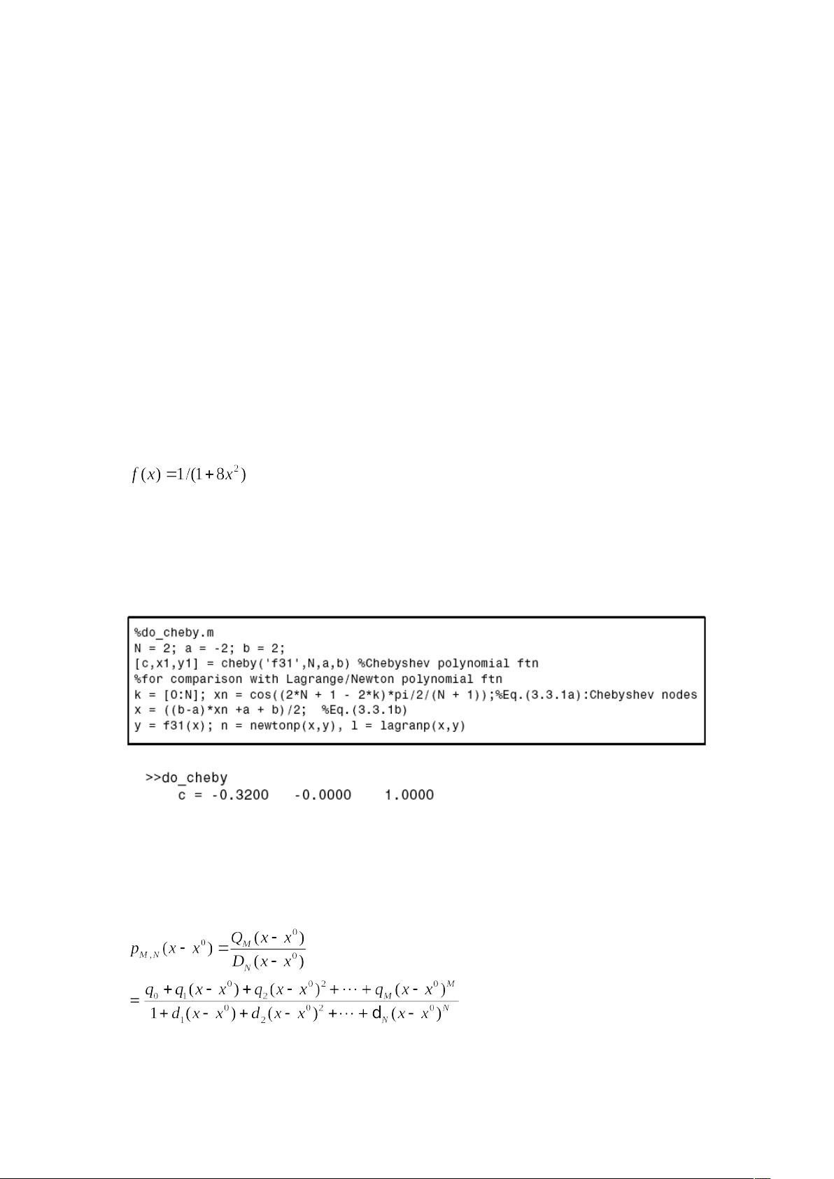
Example 3.1. Approximation by Chebyshev Polynomial. Consider the problem
of finding the second-degree (N = 2) polynomial to approximate the function
. We make the following program “do_cheby.m”, which uses
the MATLAB routine “cheby()” for this job and uses Lagrange/Newton polynomial
with the Chebyshev nodes to do the same job. Readers can run this program
to check if the results are the same.
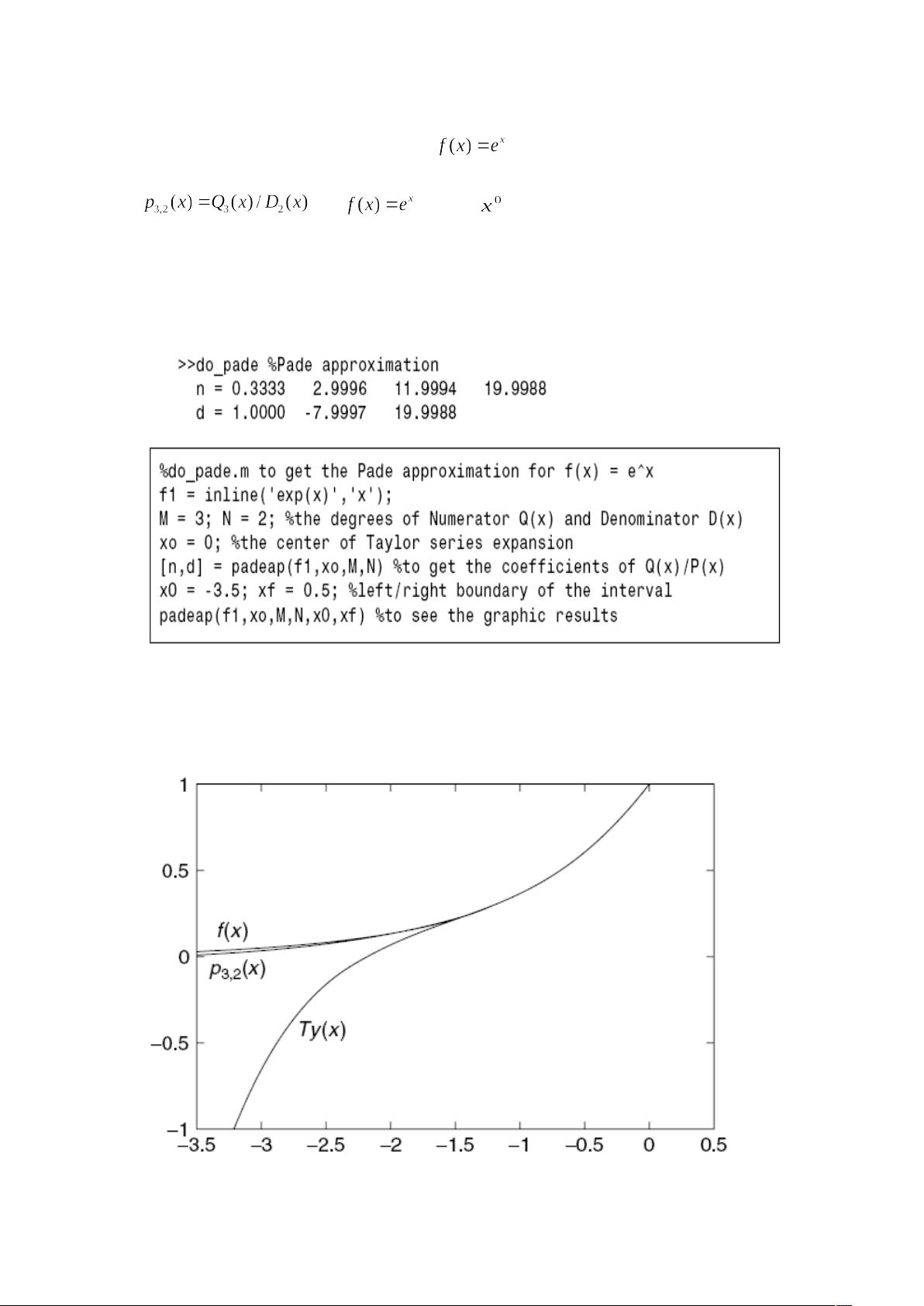
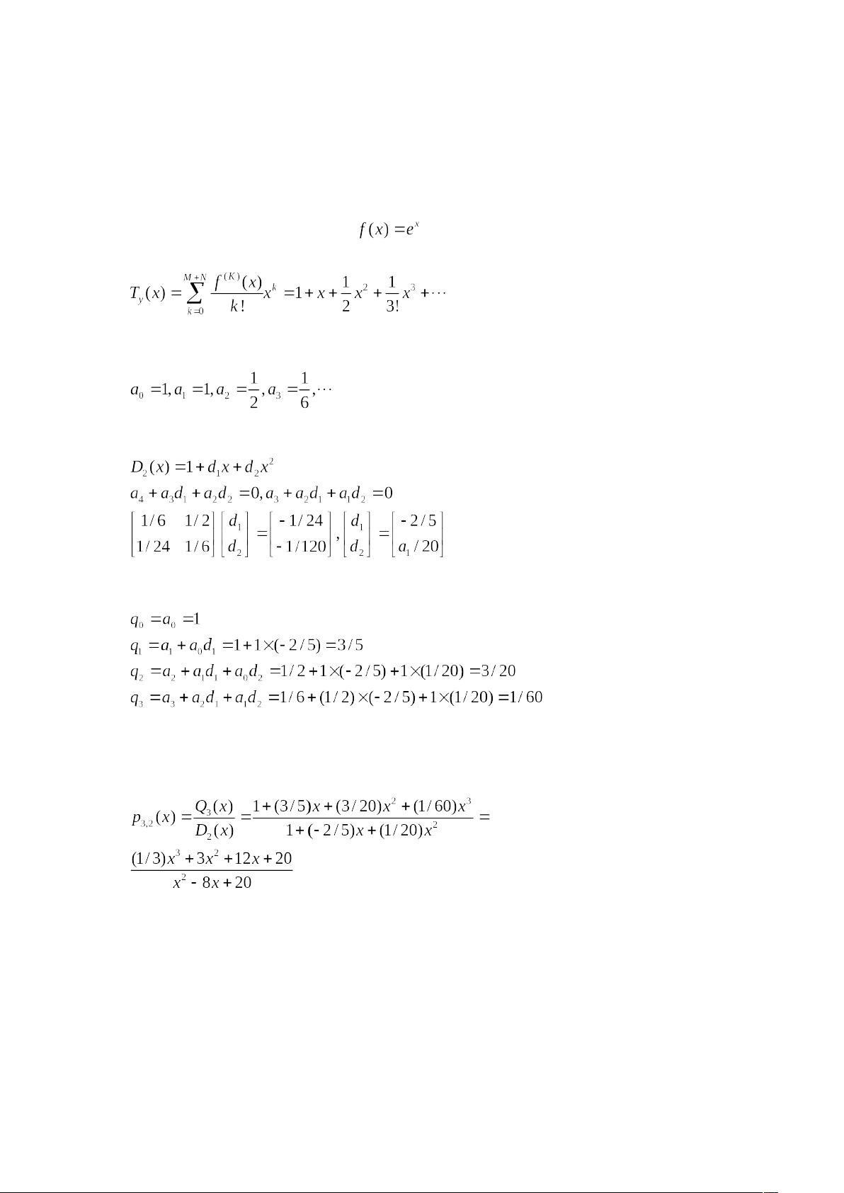
3.4 PADE APPROXIMATION BY RATIONAL FUNCTION
Pade approximation tries to approximate a function f (x) around a point xo by a
rational function
(3.4.1)
where are known.
How do we find such a rational function? We write the Taylor series expansion
of f (x) up to degree M + N at x = xo as
130 INTERPOLATION AND CURVE FITTING
Assuming =0for simplicity, we get the coefficients of
such that
(3.4.3)
by solving the following equations:
(3.4.4a)( 3.4.4b)
Here, we must first solve Eq. (3.4.4b) for and then substitute di’s
into Eq. (3.4.4a) to obtain
The MATLAB routine “padeap()” implements this scheme to find the coefficient
vectors of the numerator/denominator polynomial of the
Pade approximation for a given function f (x). Note the following things:
ž The derivatives up to order (M + N) are
computed numerically by using the routine “difapx()”, that will be introduced
in Section 5.3.
ž In order to compute the values of the Pade approximate function, we substitute
for x in which has been obtained with the assumption
that =0.
PADE APPROXIMATION BY RATIONAL FUNCTION 131
Example 3.2. Pade Approximation for . Let’s find the Pade approximation
for around =0. We make the
MATLAB program “do_pade.m”, which uses the routine “padeap()” for this
job and uses it again with no output argument to see the graphic results as
depicted in Fig. 3.6.
To confirm and support this result from the analytical point of view and to help
the readers understand the internal mechanism, we perform the hand-calculation
132 INTERPOLATION AND CURVE FITTING
Figure 3.6 Pade approximation and Taylor series expansion for f(x) = ex(Example
3.2.).
procedure. First, we write the Taylor series expansion at x = 0 up to degree
M + N = 5 for the given function as
(E3.2.1)
whose coefficients are
(E3.2.2)
We put this into Eq. (3.4.4b) with M = 3,N = 2 and solve it for di’s to get
(E3.2.3)
Substituting this to Eq. (3.4.4a) yields
(E3.2.4)
INTERPOLATION BY CUBIC SPLINE 133
With these coefficients, we write the Pade approximate function as
(E3.2.5)
3.5 INTERPOLATION BY CUBIC SPLINE
If we use the Lagrange/Newton polynomial to interpolate a given set of N + 1
data points, the polynomial is usually of degree N and so has N − 1 local extrema
(maxima/minima). Thus, it will show a wild swing/oscillation (called ‘polynomial
wiggle’), particularly near the ends of the whole interval as the number of data
剩余46页未读,继续阅读
资源评论
- weixin_410880732019-04-09跟计算机一点关系都没有
lvxiao830208
- 粉丝: 0
- 资源: 1
上传资源 快速赚钱
- 我的内容管理 展开
- 我的资源 快来上传第一个资源
- 我的收益 登录查看自己的收益
- 我的积分 登录查看自己的积分
- 我的C币 登录后查看C币余额
- 我的收藏
- 我的下载
- 下载帮助
安全验证
文档复制为VIP权益,开通VIP直接复制
信息提交成功