


Cubic Spline Interpolation
Sky McKinley and Megan Levine
Math 45: Linear Algebra
Abstract. An introduction into the theory and application of cubic splines with accompanying Matlab
m-file cspline.m
Introduction
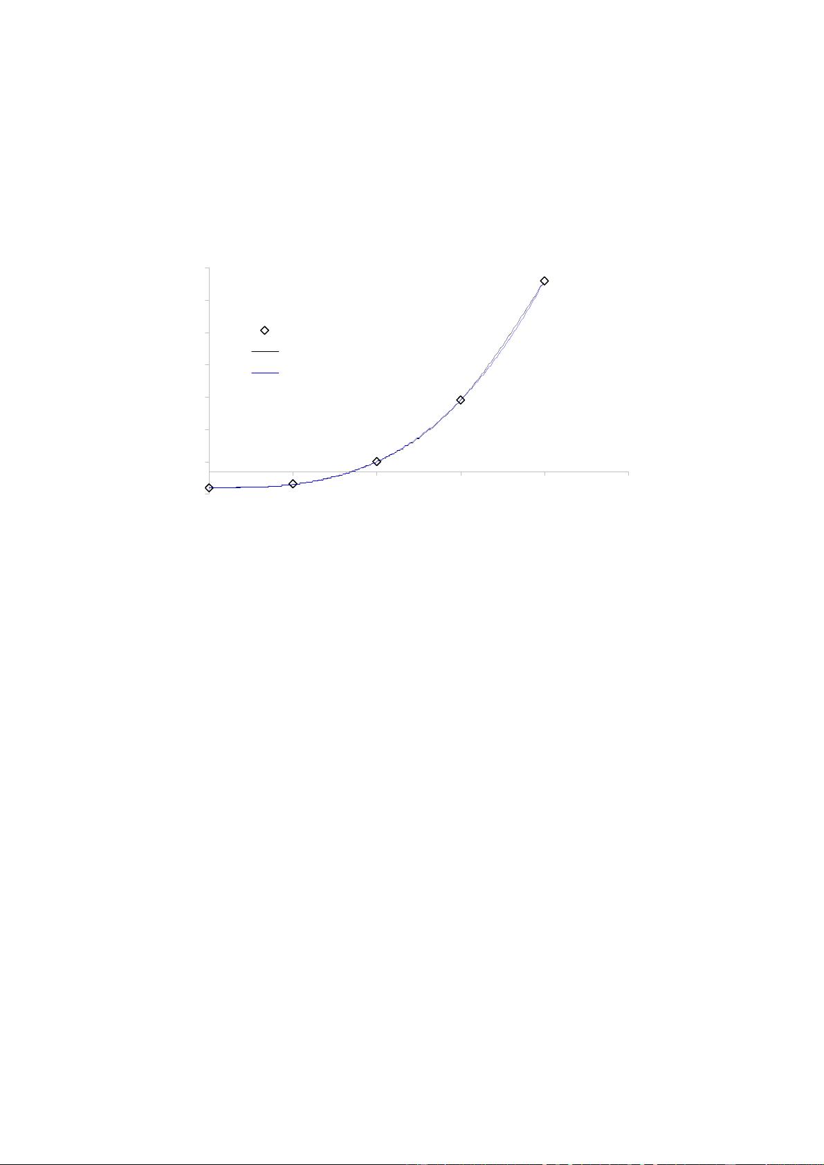
Real world numerical data is usually difficult to analyze. Any function which would
effectively correlate the data would be difficult to obtain and highly unwieldy. To this end,
the idea of the cubic spline was developed. Using this process, a series of unique cubic
polynomials are fitted between each of the data points, with the stipulation that the curve
obtained be continuous and appear smooth. These cubic splines can then be used to
determine rates of change and cumulative change over an interval. In this brief introduction,
we will only discuss splines which interpolate equally spaced data points, although a more
robust form could encompass unequally spaced points.
Theory
The fundamental idea behind cubic spline interpolation is based on the engineer’s tool
used to draw smooth curves through a number of points. This spline consists of weights
attached to a flat surface at the points to be connected. A flexible strip is then bent across
each of these weights, resulting in a pleasingly smooth curve.
The mathematical spline is similar in principle. The points, in this case, are numerical
data. The weights are the coefficients on the cubic polynomials used to interpolate the data.
These coefficients ’bend’ the line so that it passes through each of the data points without
any erratic behavior or breaks in continuity.
Process
The essential idea is to fit a piecewise function of the form
SÝxÞ =
s
1
ÝxÞ if x
1
² x < x
2
s
2
ÝxÞ if x
2
² x < x
3
_
s
n?1
ÝxÞ if x
n?1
² x < x
n
(1)
where s
i
is a third degree polynomial defined by
s
i
ÝxÞ = a
i
Ýx ? x
i
Þ
3
+ b
i
Ýx ? x
i
Þ
2
+ c
i
Ýx ? x
i
Þ + d
i
(2)
for i = 1,2,...,n ? 1.
The first and second derivatives of these n ? 1 equations are fundamental to this process,
and they are
1


- 1
- 2
- 3
前往页