没有合适的资源?快使用搜索试试~ 我知道了~
资源推荐
资源详情
资源评论

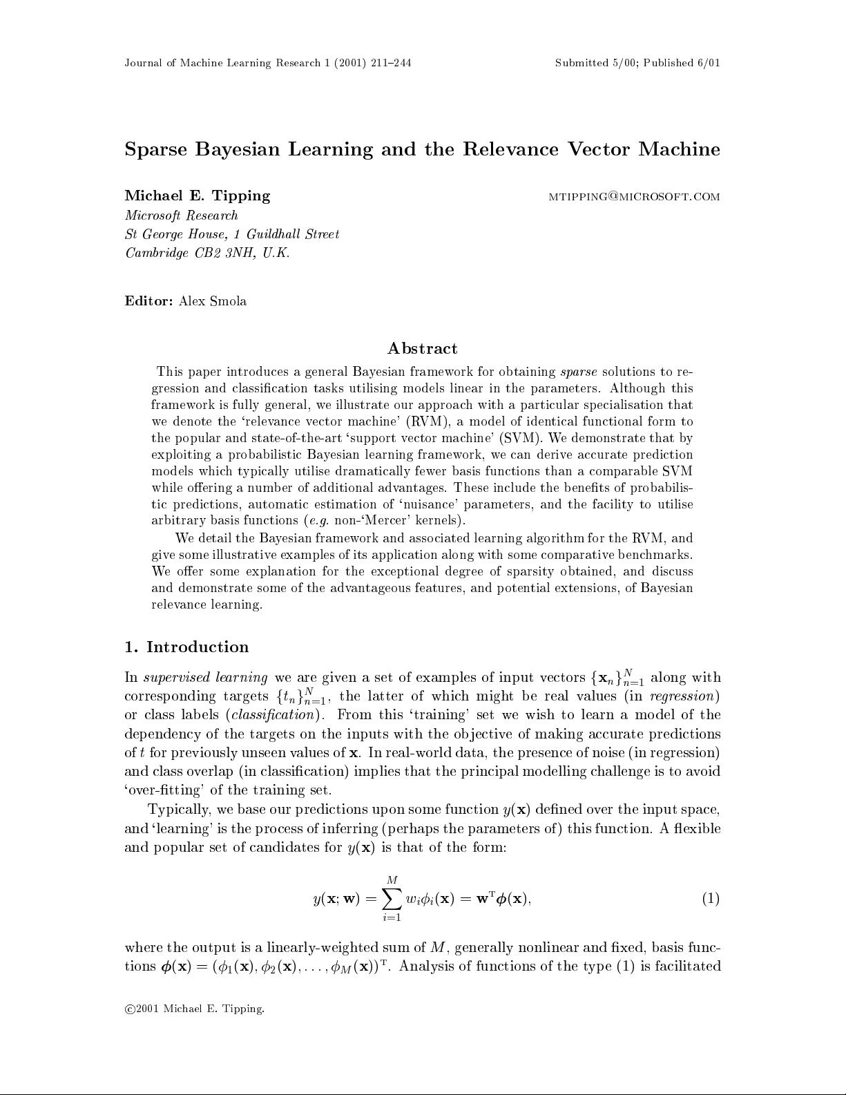
Journal of Machine Learning Research 1 (2001) 211{244 Submitted 5/00; Published 6/01
Sparse Bayesian Learning and the Relevance Vector Machine
Michael E. Tipping
mtipping@microsoft.com
Microsoft Research
St George House, 1 Guildhal l Street
Cambridge CB2 3NH, U.K.
Editor:
Alex Smola
Abstract
This paper introduces a general Bayesian framework for obtaining
sparse
solutions to re-
gression and classication tasks utilising mo dels linear in the parameters. Although this
framework is fully general, we illustrate our approach with a particular specialisation that
we denote the `relevance vector machine' (RVM), a mo del of identical functional form to
the p opular and state-of-the-art `support vector machine' (SVM). We demonstrate that by
exploiting a probabilistic Bayesian learning framework, we can derive accurate prediction
models whichtypically utilise dramatically fewer basis functions than a comparable SVM
while oering a numb er of additional advantages. These include the b enets of probabilis-
tic predictions, automatic estimation of `nuisance' parameters, and the facility to utilise
arbitrary basis functions (
e.g.
non-`Mercer' kernels).
We detail the Bayesian framework and asso ciated learning algorithm for the RVM, and
give some illustrative examples of its application along with some comparative b enchmarks.
We oer some explanation for the exceptional degree of sparsity obtained, and discuss
and demonstrate some of the advantageous features, and potential extensions, of Bayesian
relevance learning.
1. Intro duction
In
supervised learning
we are given a set of examples of input vectors
f
x
n
g
N
n
=1
along with
corresp onding targets
f
t
n
g
N
n
=1
, the latter of which might be real values (in
regression
)
or class labels (
classication
). From this `training' set we wish to learn a mo del of the
dep endency of the targets on the inputs with the ob jective of making accurate predictions
of
t
for previously unseen values of
x
. In real-world data, the presence of noise (in regression)
and class overlap (in classication) implies that the principal mo delling challenge is to avoid
`over-tting' of the training set.
Typically,we base our predictions up on some function
y
(
x
) dened over the input space,
and `learning' is the pro cess of inferring (p erhaps the parameters of ) this function. A exible
and p opular set of candidates for
y
(
x
)isthatoftheform:
y
(
x
;
w
)=
M
X
i
=1
w
i
i
(
x
)=
w
T
(
x
)
;
(1)
where the output is a linearly-weighted sum of
M
, generally nonlinear and xed, basis func-
tions
(
x
)=(
1
(
x
)
;
2
(
x
)
;:::;
M
(
x
))
T
. Analysis of functions of the typ e (1) is facilitated
c
2001 Michael E. Tipping.

Tipping
since the adjustable parameters (or `weights')
w
=(
w
1
;w
2
;:::;w
M
)
T
app ear linearly, and
the ob jective is to estimate `go o d' values for those parameters.
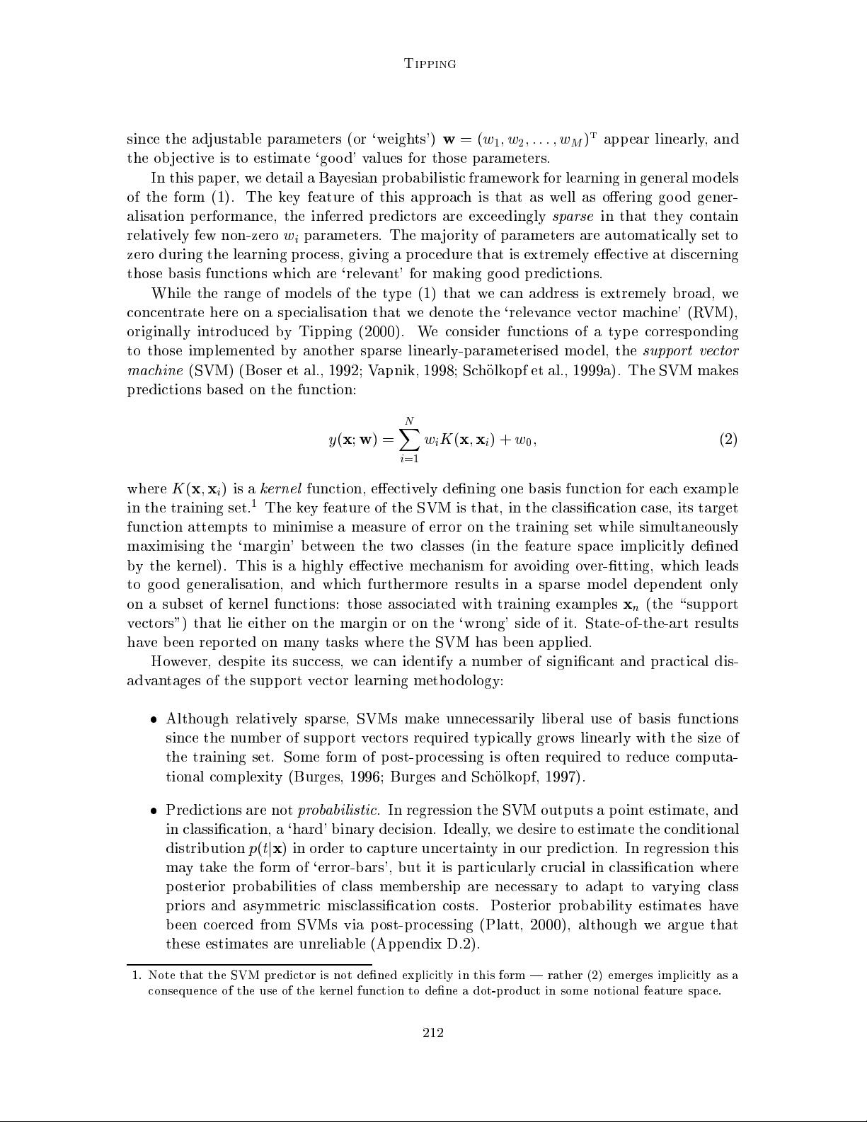
In this pap er, we detail a Bayesian probabilistic framework for learning in general mo dels
of the form (1). The key feature of this approach is that as well as oering good gener-
alisation p erformance, the inferred predictors are exceedingly
sparse
in that they contain
relatively few non-zero
w
i
parameters. The ma jority of parameters are automatically set to
zero during the learning pro cess, giving a procedure that is extremely eective at discerning
those basis functions which are `relevant' for making goo d predictions.
While the range of mo dels of the type (1) that we can address is extremely broad, we
concentrate here on a specialisation that we denote the `relevance vector machine' (RVM),
originally introduced by Tipping (2000). We consider functions of a type corresp onding
to those implemented by another sparse linearly-parameterised mo del, the
support vector
machine
(SVM) (Boser et al., 1992; Vapnik, 1998; Scholkopf et al., 1999a). The SVM makes
predictions based on the function:
y
(
x
;
w
)=
N
X
i
=1
w
i
K
(
x
;
x
i
)+
w
0
;
(2)
where
K
(
x
;
x
i
)isa
kernel
function, eectively dening one basis function for each example
in the training set.
1
The key feature of the SVM is that, in the classication case, its target
function attempts to minimise a measure of error on the training set while simultaneously
maximising the `margin' between the two classes (in the feature space implicitly dened
by the kernel). This is a highly eective mechanism for avoiding over-tting, which leads
to goo d generalisation, and which furthermore results in a sparse model dependent only
on a subset of kernel functions: those asso ciated with training examples
x
n
(the \supp ort
vectors") that lie either on the margin or on the `wrong' side of it. State-of-the-art results
have been rep orted on many tasks where the SVM has b een applied.
However, despite its success, we can identify a number of signicant and practical dis-
advantages of the supp ort vector learning methodology:
Although relatively sparse, SVMs make unnecessarily liberal use of basis functions
since the numb er of support vectors required typically grows linearly with the size of
the training set. Some form of p ost-pro cessing is often required to reduce computa-
tional complexity (Burges, 1996; Burges and Scholkopf, 1997).
Predictions are not
probabilistic
. In regression the SVM outputs a point estimate, and
in classication, a `hard' binary decision. Ideally,we desire to estimate the conditional
distribution
p
(
t
j
x
) in order to capture uncertainty in our prediction. In regression this
may take the form of `error-bars', but it is particularly crucial in classication where
p osterior probabilities of class memb ership are necessary to adapt to varying class
priors and asymmetric misclassication costs. Posterior probability estimates have
b een co erced from SVMs via p ost-pro cessing (Platt, 2000), although we argue that
these estimates are unreliable (App endix D.2).
1. Note that the SVM predictor is not dened explicitly in this form | rather (2) emerges implicitly as a
consequence of the use of the kernel function to dene a dot-product in some notional feature space.
212

Sparse Bayesian Learning and the Relevance Vector Machine
It is necessary to estimate the error/margin trade-o parameter `
C
' (and in regression,
the insensitivity parameter `
'too). This generally entails a cross-validation pro cedure,
whichis wasteful b oth of data and computation.
The kernel function
K
(
x
;
x
i
)must satisfy Mercer's condition. That is, it must b e the
continuous symmetric kernel of a positiveintegral operator.
2
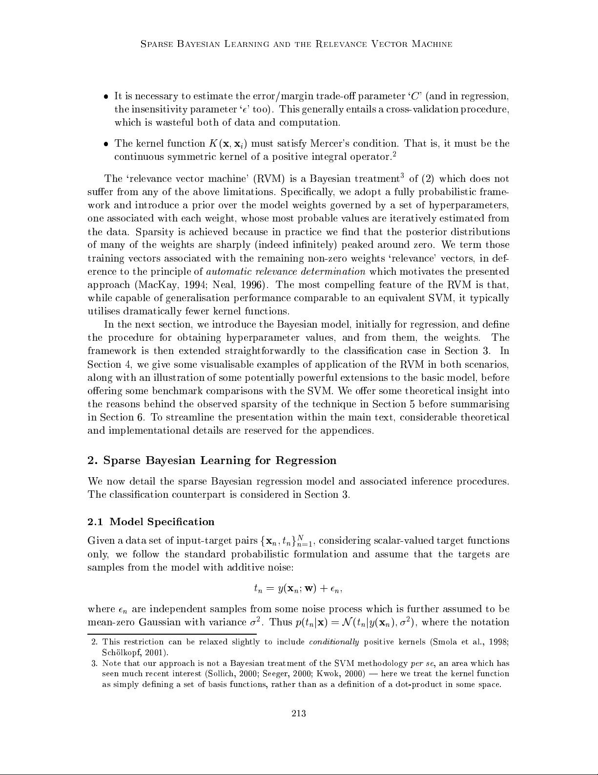
The `relevance vector machine' (RVM) is a Bayesian treatment
3
of (2) which do es not
suer from anyoftheabove limitations. Sp ecically,we adopt a fully probabilistic frame-
work and intro duce a prior over the mo del weights governed by a set of hyp erparameters,
one associated with eachweight, whose most probable values are iteratively estimated from
the data. Sparsity is achieved b ecause in practice we nd that the p osterior distributions
of many of the weights are sharply (indeed innitely) peaked around zero. We term those
training vectors associated with the remaining non-zero weights `relevance' vectors, in def-
erence to the principle of
automatic relevance determination
whichmotivates the presented
approach (MacKay, 1994; Neal, 1996). The most comp elling feature of the RVM is that,
while capable of generalisation performance comparable to an equivalent SVM, it typically
utilises dramatically fewer kernel functions.
In the next section, weintro duce the Bayesian mo del, initially for regression, and dene
the pro cedure for obtaining hyperparameter values, and from them, the weights. The
framework is then extended straightforwardly to the classication case in Section 3. In
Section 4, wegive some visualisable examples of application of the RVM in both scenarios,
along with an illustration of some p otentially p owerful extensions to the basic mo del, b efore
oering some b enchmark comparisons with the SVM. We oer some theoretical insightinto
the reasons b ehind the observed sparsity of the technique in Section 5 before summarising
in Section 6. To streamline the presentation within the main text, considerable theoretical
and implementational details are reserved for the app endices.
2. Sparse Bayesian Learning for Regression
We now detail the sparse Bayesian regression mo del and asso ciated inference pro cedures.
The classication counterpart is considered in Section 3.
2.1 Mo del Sp ecication
Given a data set of input-target pairs
f
x
n
;t
n
g
N
n
=1
, considering scalar-valued target functions
only, we follow the standard probabilistic formulation and assume that the targets are
samples from the model with additive noise:
t
n
=
y
(
x
n
;
w
)+
n
;
where
n
are indep endent samples from some noise process which is further assumed to be
mean-zero Gaussian with variance
2
. Thus
p
(
t
n
j
x
)=
N
(
t
n
j
y
(
x
n
)
;
2
), where the notation
2. This restriction can be relaxed slightly to include
conditional ly
positive kernels (Smola et al., 1998;
Scholkopf, 2001).
3. Note that our approachisnotaBayesian treatment of the SVM metho dology
per se
, an area which has
seen much recentinterest (Sollich, 2000; Seeger, 2000; Kwok, 2000) | here we treat the kernel function
as simply dening a set of basis functions, rather than as a denition of a dot-pro duct in some space.
213

Tipping
sp ecies a Gaussian distribution over
t
n
with mean
y
(
x
n
) and variance
2
. The function
y
(
x
) is as dened in (2) for the SVM where weidentify our general basis functions with the
kernel as parameterised by the training vectors:
i
(
x
)
K
(
x
;
x
i
). Due to the assumption
of indep endence of the
t
n
, the likeliho o d of the complete data set can b e written as
p
(
t
j
w
;
2
)=(2
2
)
N=
2
exp
1
2
2
k
t
w
k
2
;
(4)
where
t
=(
t
1
:::t
N
)
T
,
w
=(
w
0
:::w
N
)
T
and
is the
N
(
N
+ 1) `design' matrix with
=
[
(
x
1
)
;
(
x
2
)
;:::;
(
x
N
)]
T
, wherein
(
x
n
)=[1
;K
(
x
n
;
x
1
)
;K
(
x
n
;
x
2
)
;:::;K
(
x
n
;
x
N
)]
T
. For
clarity, we omit to notate the implicit conditioning upon the set of input vectors
f
x
n
g
in
(4) and subsequent expressions.
With as many parameters in the mo del as training examples, wewould exp ect maximum-
likeliho o d estimation of
w
and
2
from (4) to lead to severe over-tting. To avoid this, a
common approach is to imp ose some additional constraint on the parameters, for example,
through the addition of a `complexity' p enalty term to the likeliho o d or error function. This
is implicitly eected by the inclusion of the `margin' term in the SVM. Here, though, we
adopt a Bayesian persp ective, and `constrain' the parameters by dening an explicit
prior
probability distribution over them.
We enco de a preference for smo other (less complex) functions by making the p opular
choice of a zero-mean Gaussian prior distribution over
w
:
p
(
w
j
)=
N
Y
i
=0
N
(
w
i
j
0
;
1
i
)
;
(5)
with
a vector of
N
+1
hyperparameters
. Importantly, there is an individual hyperpa-
rameter asso ciated indep endently with every weight, mo derating the strength of the prior
thereon.
4
To complete the sp ecication of this
hierarchical
prior, we must dene hyperpriors
over
, as well as over the nal remaining parameter in the model, the noise variance
2
.
These quantities are examples of
scale
parameters, and suitable priors thereover are Gamma
distributions (see,
e.g.
, Berger, 1985):
p
(
)=
N
Y
i
=0
Gamma(
i
j
a; b
)
;
p
(
) = Gamma(
j
c; d
)
;
with
2
and where
Gamma(
j
a; b
)=(
a
)
1
b
a
a
1
e
b
;
(6)
with (
a
)=
R
1
0
t
a
1
e
t
dt
, the `gamma function'. Tomake these priors non-informative(
i.e.
at), we might x their parameters to small values:
e.g.
a
=
b
=
c
=
d
=10
4
. However, by
4. Note that although it is not a characteristic of this parameter prior in general, for the case of the RVM
that we consider here, the overall implied prior over functions is
data dependent
due to the app earance
of
x
n
in the basis functions
K
(
x
;
x
n
). This presents no practical diÆculty, although wemust take care in
interpreting the \error-bars" implied by the model. In Appendix D.1 we consider this in further detail.
214

Sparse Bayesian Learning and the Relevance Vector Machine
setting these parameters to zero, we obtain uniform hyp erpriors (over a
logarithmic
scale).
Since all scales are equally likely, a pleasing consequence of the use of such `improp er'
hyp erpriors here is that of scale-invariance: predictions are indep endent of linear scaling of
both
t
and the basis function outputs so, for example, results do not dep end on the unit
of measurement of the targets. For completeness, the more detailed derivations oered in
App endix A will consider the case of general Gamma priors for
and
, but in the main
b o dy of the pap er, all further analysis and presented results will assume uniform scale priors
with
a
=
b
=
c
=
d
=0.
This formulation of prior distributions is a type of
automatic relevance determination
(ARD) prior (MacKay, 1994; Neal, 1996). Using such priors in a neural network, individual
hyp erparameters would typically control
groups
of weights | those associated with each
input dimension
x
(this idea has also been applied to the input variables in `Gaussian
pro cess' mo dels). Should the evidence from the data support such a hyp othesis, using a
broad prior over the hyp erparameters allows the p osterior probability mass to concentrate
at very large values of some of these
variables, with the consequence that the p osterior
probability of the associated weights will b e concentrated at zero, thus eectively `switching
o ' the corresp onding inputs, and so deeming them to b e `irrelevant'.
Here, the assignment of an individual hyperparameter to eachweight, or basis function,
is the key feature of the relevance vector machine, and is resp onsible ultimately for its
sparsity properties. To intro duce an additional
N
+1 parameters to the mo del may seem
counter-intuitive, since we have already conceded that we have to o many parameters, but
from a Bayesian p ersp ective, if we correctly `integrate out' all such `nuisance' parameters
(or can approximate such a pro cedure suÆciently accurately), then this presents no problem
from a methodological persp ective (see Neal, 1996, pp. 16{17). Any subsequently observed
`failure' in learning is attributable to the form, not the parameterisation, of the prior over
functions.
2.2 Inference
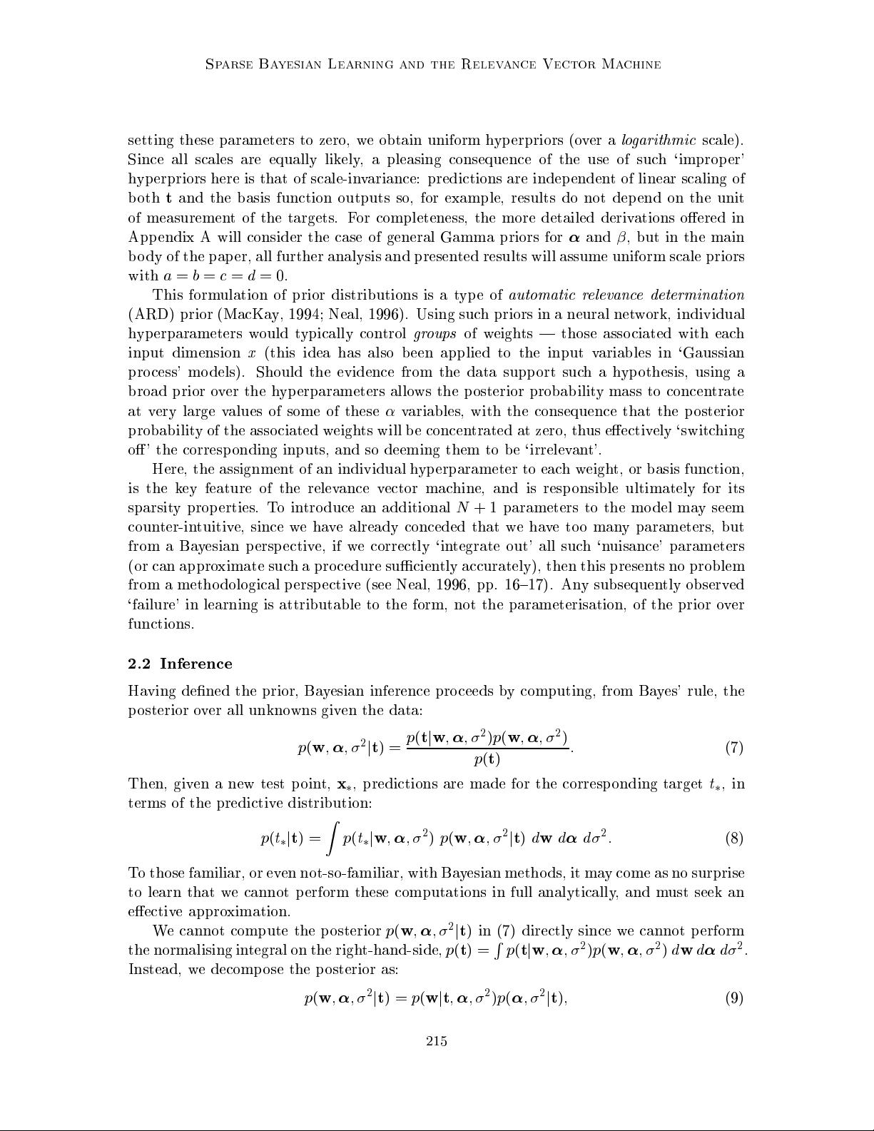
Having dened the prior, Bayesian inference pro ceeds by computing, from Bayes' rule, the
p osterior over all unknowns given the data:
p
(
w
;
;
2
j
t
)=
p
(
t
j
w
;
;
2
)
p
(
w
;
;
2
)
p
(
t
)
:
(7)
Then, given a new test point,
x
, predictions are made for the corresp onding target
t
, in
terms of the predictive distribution:
p
(
t
j
t
)=
Z
p
(
t
j
w
;
;
2
)
p
(
w
;
;
2
j
t
)
d
w
d
d
2
:
(8)
To those familiar, or even not-so-familiar, with Bayesian metho ds, it may come as no surprise
to learn that we cannot p erform these computations in full analytically, and must seek an
eectiveapproximation.
We cannot compute the p osterior
p
(
w
;
;
2
j
t
) in (7) directly since we cannot p erform
the normalising integral on the right-hand-side,
p
(
t
)=
R
p
(
t
j
w
;
;
2
)
p
(
w
;
;
2
)
d
w
d
d
2
.
Instead, we decomp ose the posterior as:
p
(
w
;
;
2
j
t
)=
p
(
w
j
t
;
;
2
)
p
(
;
2
j
t
)
;
(9)
215
剩余33页未读,继续阅读
资源评论

cauchy
- 粉丝: 1
- 资源: 5
上传资源 快速赚钱
 我的内容管理
展开
 我的资源
快来上传第一个资源
 我的收益 登录查看自己的收益
 我的积分
登录查看自己的积分
 我的C币
登录后查看C币余额
 我的收藏
我的收藏  我的下载
我的下载  下载帮助
下载帮助

 前往需求广场,查看用户热搜
最新资源
资源上传下载、课程学习等过程中有任何疑问或建议,欢迎提出宝贵意见哦~我们会及时处理!
点击此处反馈


安全验证
文档复制为VIP权益,开通VIP直接复制
 信息提交成功