


Middle East Technical University
EE498 Control System Design and
Simulation Term Project
June 9, 2018
MPC of Permanent Magnet Synchronous
Generator with 2 L-VSI Grid-Side and Passive
Generator Side Converters of a Wind Turbine
Asena Melisa SARICI-2031284
supervised by
Claus Werner Schmidt
Contents
1 Introduction 1
2 Mathematical Model 1
3 System Constraints and Parameters 4
4 MATLAB Model Predictive Control Implementation 5
5 Simulink 9
6 Conclusion 11
References 12
7 Appendix 13
1 Introduction
This project focuses on Model Predictive Current Control Application for a surface mount
permanent magnet synchronous machine wind turbine. The model used is the electrical
model for the machine. Considering the complicated and highly nonlinear aerodynamic
system of the wind turbines,the focus is chosen as the power converters. MPC is a
relatively new application in power electronics yet a promising control method. The
simplified model of the turbine is provided and the MPC code is generated in MATLAB
and Simulink.
2 Mathematical Model
[1],[3], [7],[4], [5]
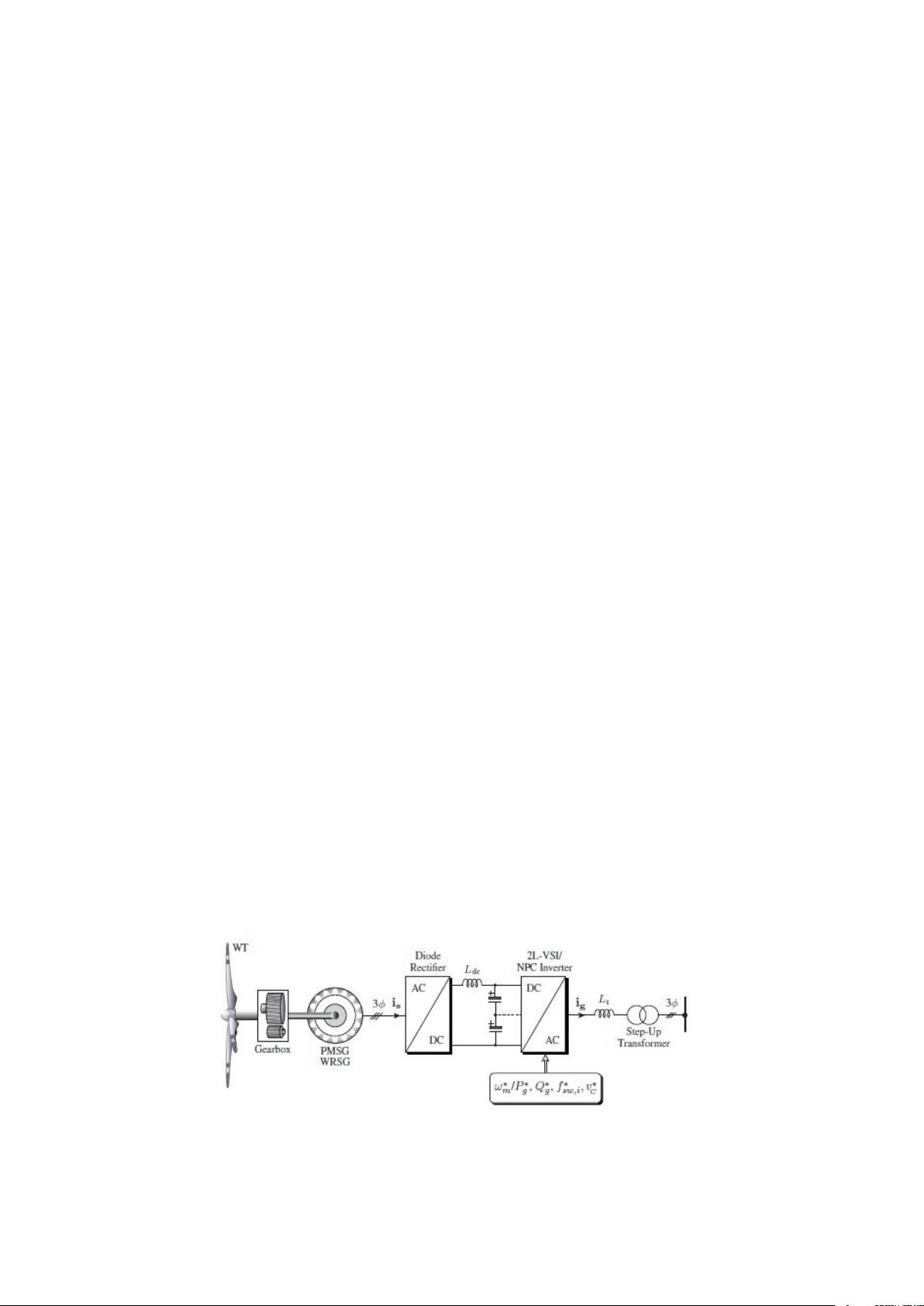
A Wind Turbine Model is seen in figure 1. The model power converter topology
contains a diode rectifier for rectifying the AC voltage to DC first in order to change
the frequency and magnitude of the generator side and integrate generator side 3 phase
to grid side. DC link voltage is connected to a 2 level Voltage Source Inverter whose
configuration can be seen in figure 2.
Figure 1: Passive Generator Side and 2LVSI Grid Side SPMG [8]
1

Figure 2: Detailed Circuit Configuration for Passive Generator Side and 2LVSI Grid Side
SPMG [8]
For the models given above, the voltage of the grid side is determined by the switching
sequence applied to the generator. From now on, in order to simplify the MPC computa-
tions dq frame will be used for currnent and voltage waveforms. For this abc to dq frame
Park Transformation is used.
In order to understand this concept, let us consider the abc and dq frame illustration
shown in figure 5.
Figure 3: Representation of abcand dq frames of SPMG and angular correspondence[8]
Hence, the dq voltages will be the inputs of the mathematical model to be built,
whereas the dq frame currents will be the state variables. The output to be observed can
be selected anything. However, since the cost function is built in order to maximize the
real power and minimize the reactive power, which are directly related with d and q axis
currents respectively, the power is selected to be the output to be observed.
It is also important to note that the wind turbine can operate in 4 quadrants as seen
in 4. Once again, for simplicity we will assume that the operation is in 2nd quadrant
which is the generation mode.
2
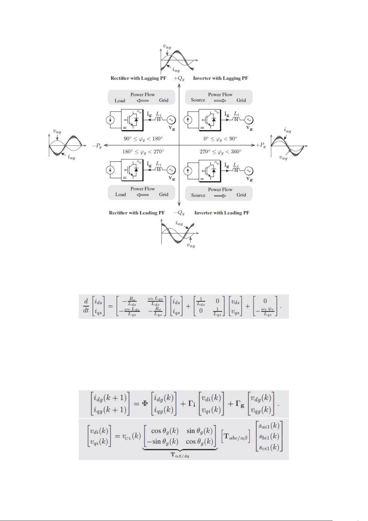
Figure 4: 4 Quadrant Operation for the Wind Turbine [8]
The continuous time model for the stator side (before the rectifier) is:
Figure 5: Stator Side Continuous Time Model [8]
For a surfacemount machine L
d
sand L
q
s are the same. A similar model for the grid
side 3 phase is accurate. As seen, the model depends on the rotor speed, which for
simplicity, will be assumed as constant.
Similarly, the grid side discrete time current representation is shown in ??
Figure 6: Grid Side General Discrete Time Model [8]
3
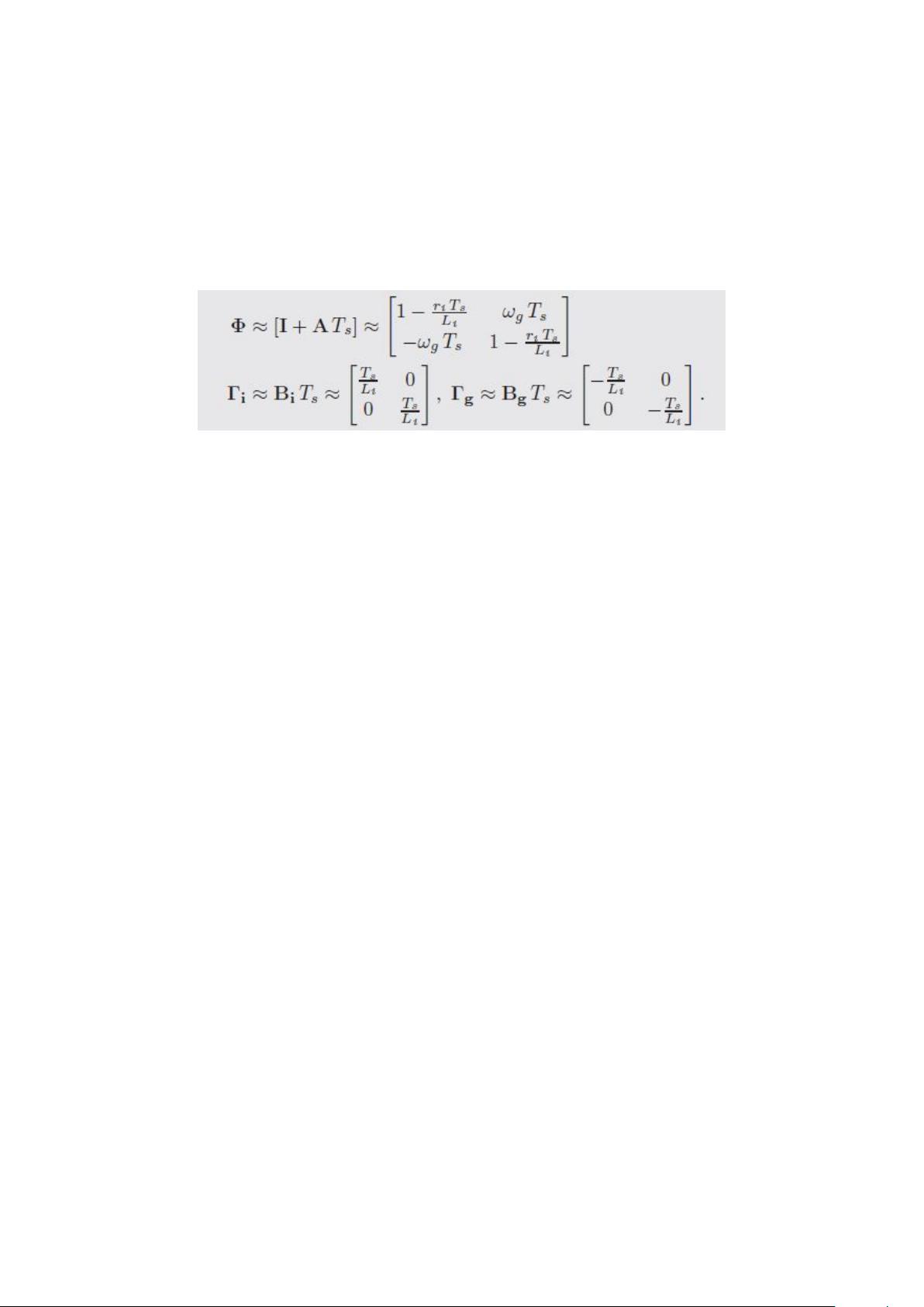
In the above equation the subscript g represents the grid and i represents the inverter.
As mentioned the inverter voltages are controlled with 8 space vector switches and these
switch states with the rotational angle decide the dq voltages at a given time and they
are the input of the above 6. Moreover, the grid side voltage is assumed to be a stable
constant bus and will be assumed to be constant (and will be subtracted from the inverter
side voltage v
d/qi
like a a reference frame). Following estimations 7 are used according to
[8]
Figure 7: Grid Side General Discrete Time Model Matrices’ Estimations [8]
• Calculation of Reference Currents
dq axis reference currents will be obtained from the DC side.
• Prediction of Future Behaviour of the Grid Currents
This behaviour will be obtained from Model Predictive Control
• Cost Function
Regulation of the active power is dependent on the d-axis current, whereas the
reactive power depends on q-axis current. Switching frequency minimisation will
be eliminated for simplicity and cost function will be generated for maximising the
real power output.
In the lectures, we have generated the linear quadratic regulation to decrease the states
to 0 and formed the objective functions accordingly, hence the output converges to 0 as
well. For a wind turbine system, however, it is important to note here that we have taken
the grid current as our state variable whose d axis current is desired to have a nonzero
value for keeping our power constant, which should have a nonzero constant value for
all the time. Therefore, the cost function wants to minimise the difference between the
reference grid currents and the actual grid currents. Therefore, converging to 0 will be
accepted as converging to the reference value. This goal can be expressed as in equation
1.
G(k) = λ
id
[(i
dref
(k + 1) − i
dpredicted
(k + 1))
2
] + λ
iq
[(iqref(k + 1) − i
qpredicted
(k + 1))
2
] (1)
3 System Constraints and Parameters
There are a number of different wind turbine generator types with different power speci-
fications. Using a passive generator side machine I have selected a low power machine for
modelling and its parameters to be used are shown in the table1.
4


