


Introduction to Digital Signal Processing and Digital Filtering
1.1 Introduction
Digital signal processing (DSP) refers to anything that can be done to a
signal using code on a computer or DSP chip. To reduce certain
sinusoidal frequency components in a signal in amplitude, digital filtering
is done. One may want to obtain the integral of a signal. If the signal
comes from a tachometer, the integral gives the position. If the signal is
noisy, then filtering the signal to reduce the amplitudes of the noise
frequencies improves signal quality. For example, noise may occur from
wind or rain at an outdoor music presentation. Filtering out sinusoidal
components of the signal that occur at frequencies that cannot be
produced by the music itself results in recording the music with little wind
and rain noise. Sometimes the signal is corrupted not by noise, but by
other signal frequencies that are of no present interest. If the signal is an
electronic measurement of a brain wave obtained by using probes applied
externally to the head, other electronic signals are picked up by the
probes, but the physician may be interested only in signals occurring at a
particular frequency. By using digital filtering, the signals of interest only
can be presented to the physician.
1.2 Historical Perspective
Originally signal processing was done only on analog or continuous time
signals using analog signal processing (ASP). Until the late 1950s digital
Introduction to Digital Signal
Processing and Digital Filtering
chapter
1
1

computers were not commercially available. When they did become
commercially available they were large and expensive, and they were used
to simulate the performance of analog signal processing to judge its
effectiveness. These simulations, however, led to digital processor code
that simulated or performed nearly the same task on samples of the
signals that the analog systems did on the signal. After a while it was
realized that the simulation coding of the analog system was actually a
DSP system that worked on samples of the input and output at discrete
time intervals.
But to implement signal processing digitally instead of using analog
systems was still out of the question. The first problem was that an analog
input signal had to be represented as a sequence of samples of the signal,
which were then converted to the computer’s numerical representation.
The same process would have to be applied in reverse to the output of
the digitally processed signal. The second problem was that because the
processing was done on very large, slow, and expensive computers,
practical real-time processing between samples of the signal was impossi-
ble. Finally, as we will see in Chapter 9, even if digital processing could
be done quickly enough between input samples in order to adequately
represent the input signal, high sample rates require more bits of
precision than slower ones.
The development of faster, cheaper, and smaller input signal samplers
(ADCs) and output converters from digital data to analog data (DACs)
began to make real-time DSP practical. Also, the processors were
becoming smaller, faster, and cheaper and used more bits. Real-time
replacements for analog systems may be just as small, cheap, and accurate
and be able to process at a sample rate adequate for many analog signals.
However, testing and modification of the coding for DSP systems led to
DSP systems that have no analog signal processing equivalents, yet
sometimes perform the signal processing better than the DSP coding
developed to replace analog systems. For digital filtering, these processing
methods are discussed in Chapters 10 and 11.
1.3 Simple Examples of Digital Signal Processing
Digital signal processing entails anything that can be done to a signal
using coding on a computer or DSP chip. This includes digital filtering
2
Digital Signal Processing
of signals as well as digital integration and digital correlation of signals.
This text concentrates on constant rate digital filtering, with references
to where the material is applicable to DSP in general. At the end of the
text the techniques developed for digital filtering will be used for the DSP
task of integration to show how the concepts and techniques are not
limited to digital filtering.
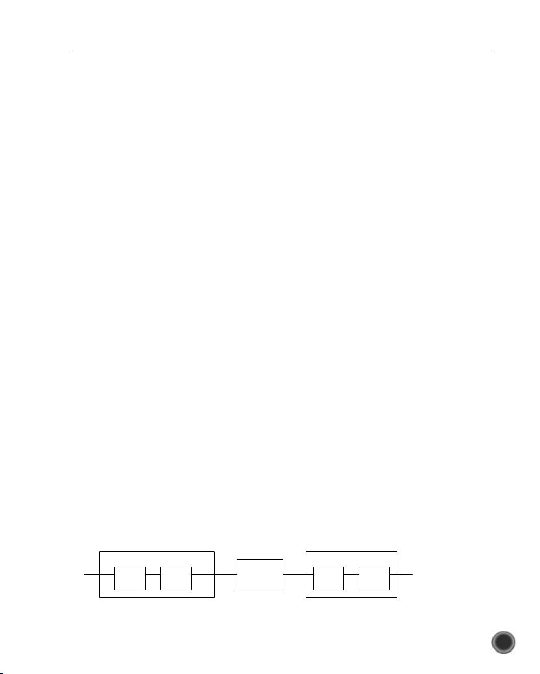
The concepts are very simple. A signal is sampled in time at a constant rate
in order to input its magnitude value at periodic intervals into the com-
puter. The sample value of the analog magnitude is converted into a binary
number. The sampling and conversion are done with an analog to digital
converter (ADC). Now the computer code can work on the signal. The
computer code computes an output value, which is converted to an analog
magnitude from a binary number and then held constant until a new out-
put is computed to replace it. This is done by a digital to analog converter
(DAC). The basic DSP system described here is shown in Figure 1.1.
To illustrate the concept of DSP and to see where more study and analysis
are needed, let’s look at a few simple things that can be done to a sampled
signal. If a signal is sampled every T seconds by an ADC and in the
computer the sample value is just multiplied by a constant and then sent
to the DAC, you have a digital amplifier. The gain of the amplifier is equal
to the coded value of the constant. The following equation describes this
digital amplifier, where x is the current input sample value from the ADC
and y is the corresponding computer output to the DAC.
y = ax A simple digital amplifier
If the sampled value of the input signal is multiplied by T , you have
computed an approximation to the area under the signal between
samples, as long as the signal doesn’t change too much between samples.
If this value is added to the previous input sample multiplied by T , you
3
sampler analog/bin
computer
coding
bin/analog hold
ADC DAC
x(t)
xy
y(t)
Figure 1.1. Basic DSP system
Introduction to Digital Signal Processing and Digital Filtering

have approximated the area under the signal over two sample times. This
could be repeated endlessly to approximate the area under the signal
from when sampling started, as shown in Figure 1.2. The area under a
signal or function is its integral. Thus you have performed very simple
digital integration using the current sample of the input multiplied by T
and then adding the result to the previous output. This process is
described by the following equations after two input samples (the –1
subscripts indicate they are previous input or output values).
y
–1
= Tx
–1
Simple digital integration after one input sample
(the previous sample)
y = y
–1
+ Tx Simple digital integration after two input samples
(the current sample)
By using looping, such as a “While” or “For” loop, the preceding
equations could be repeated endlessly by looping about one equation.
If the current input sample value is multiplied by one-half and added to
half the previous sample value of the input, a current change in the input
signal is reduced, while if the signal is changing slowly the output is very
close to the input, since it is just the sum of two half values. Thus the
computer is doing a very simple lowpass filtering of the input signal. This
simple process is represented by the following equation. The result of
using this equation on a string of input samples from the ADC is the input
to the DAC shown in Table 1.1. As can be seen, the results, y, are
smoothed or lowpass filtered versions of x, the ADC output.
y = 0.5x + 0.5x
–1
Simple digital lowpass filtering
4
x(t)
t
T2T 3T
area under dashed boxes approximates
area under x(t) after 2 samples at t = 0 and t = T
x(0)
x(T)
x(2T)
Figure 1.2. Example of digital integration
Digital Signal Processing


