


nauty and Traces User’s Guide (Version 2.6)
Brendan D. McKay
∗
Research School of Computer Science
Australian National University
Canberra ACT 0200, Australia
Adolfo Piperno
Departimento di Informatica
Sapienza Universit`a di Roma
Rome, Italy
August 19, 2016
Contents
0. How to use this Guide.
1. Introduction.
2. The dreadnaut program.
3. Data structures.
4. Size limits.
5. Options and statistics.
6. Calling nauty and Traces.
7. Description of the procedure parameters.
8. Interpretation of the output.
9. User-defined procedures.
10. Vertex-invariants.
11. Writing programs which call dense nauty.
12. Writing programs which call sparse nauty.
13. Writing programs which call Traces.
14. Variations.
15. Utilities (gtools).
16. Installing nauty and Traces.
17. Recent changes.
18. More on automorphism groups.
19. Graph formats used by the utilities.
20. Other ways to use nauty.
21. Licence details.
22. Acknowledgements.
23. Help texts for the utilities.
– References.
∗
Research supported by the Australian Research Council.
1

0 How to use this Guide
nauty (no automorphisms, yes?) is a set of procedures for determining the automorphism
group of a vertex-coloured graph, and for testing graphs for isomorphism. Traces is an
alternative program for these operations.
The dreadnaut program provides sufficient functionality that most simple applica-
tions can be managed without the need to write any programs. Section 2 is intended to
be a fairly self-contained introduction to that level of use. You should start by reading
Section 1 and Section 2.
nauty and Traces also come with a set of utilities suitable for processing files of
graphs; these are described in Section 15.
For other serious purposes, you will need to write a program that calls nauty or
Traces. In that case you don’t have much choice but to read this Guide from start to
finish. However, it isn’t really as hard as it sounds; see the sample programs in this guide
for a constructive proof.
The current versions of nauty and Traces are available at
http://cs.anu.edu.au/∼bdm/nauty and http://pallini.di.uniroma1.it. There is
also a mailing list you can subscribe to if you want to discuss nauty and Traces and
receive upgrade notices: http://mailman.anu.edu.au/mailman/listinfo/nauty.
nauty and Traces are written in a highly portable subset of the language C. Modern
C compilers for most types of computer should be able to handle them without difficulty.
The theoretical basis of the original edition of nauty first appeared in [9]. An updated
account, and a detailed description of Traces appears in [10].
1 Introduction
nauty and Traces come with a primitive interactive interface dreadnaut which will
suffice for most one-off computations. This chapter describes the basic concepts and gives
examples of dreadnaut usage. Later chapters will describe the programming interface.
A graph for our purposes has a finite set of vertices, and a finite set of edges. Most of
the time when we write “graph” we mean “simple undirected graph”, which implies that
each edge is an unordered pair vw of distinct vertices (so multiple edges and loops are
not included).
The following shows a graph with 8 vertices and 12 edges.
4
5
1
3
2
7
6
0
An automorphism of a graph is a permutation of the vertex labels so that the set of
2
edges remains the same. In the above graph we can interchange vertex labels 0,1 and
interchange vertex labels 2,3, and this preserves the edge set (for example, 2 is adjacent
to 5 before and after, while 0 is not adjacent to 4 before or after). This means that
(0 1)(2 3) is an automorphism.
(0 1)(2 3)
4
5 7
6
2
3
1
0
4
5
1
3
2
7
6
0
The application of two automorphisms one after the other is an automorphism too.
The set of all automorphisms, including the trivial one (that moves no labels at all), is
called the automorphism group of the graph. The automorphism group of the graph above
has 8 automorphisms:
(1) (0 6)(1 7)(2 4)(3 5)
(0 1)(2 3) (0 7)(2 5)(1 6)(3 4)
(4 5)(6 7) (0 6 1 7)(2 4 3 5)
(0 1)(2 3)(4 5)(6 7) (0 7 1 6)(2 5 3 4)
Because the number of automorphisms can be extremely large, it is more efficient to
work with a set of generators of the automorphism group. This is a set of automorphisms
such that every automorphism can be expressed as a combination of them. In the example,
a set of generators is {(4 5)(6 7), (0 6)(1 7)(2 4)(3 5)}.
The automorphisms also define an equivalence relationship on the vertices of the graph:
two vertices are equivalent if there is an automorphism taking one to the other. For
example, vertices 6 and 7 are equivalent since the automorphism (4 5)(6 7) takes 6 onto 7.
The sets of equivalent vertices are called orbits; in the example they are {0, 1, 6, 7} and
{2, 3, 4, 5}.
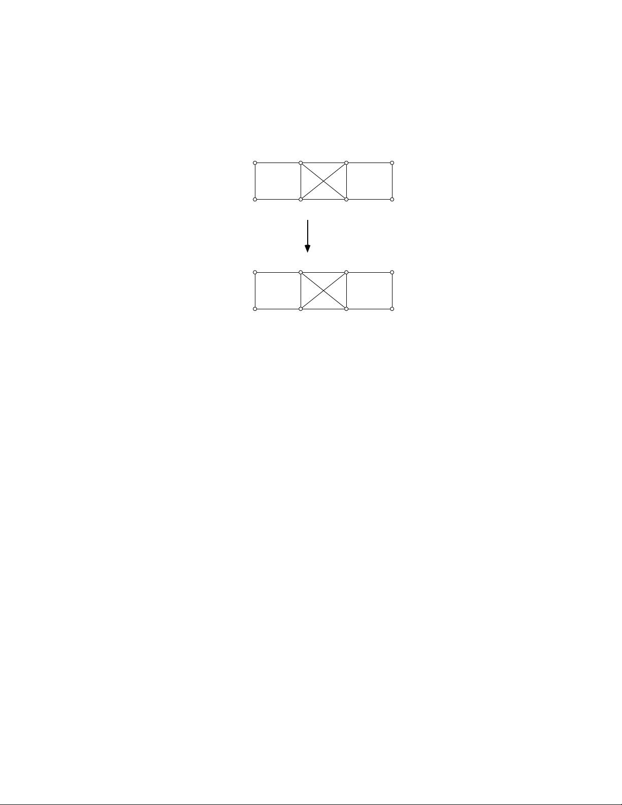
Another function that nauty and Traces can perform is canonical labelling. This is
an operation of placing the vertex labels in a way that does not depend on where they were
before. Graphs that are isomorphic (the same except for vertex labels) become identical
(exactly the same) after canonical labelling (canonizing).
In the figure below, the two graphs in the upper row are clearly isomorphic, though
they are not identical (for example 0 and 4 are adjacent in the left graph but not in the
right graph). However, when the graphs are canonized, producing the graphs in the lower
3
row, the results are identical (note that the edges of the two graphs are the same, even
though the drawings differ).
canonize
canonize
different
same
1
2
7
4
0
5
3
6
0
1
2
4
5
6
73
5
6
7
2
3
4
0
1
5 3
1
0
7
6
2
4
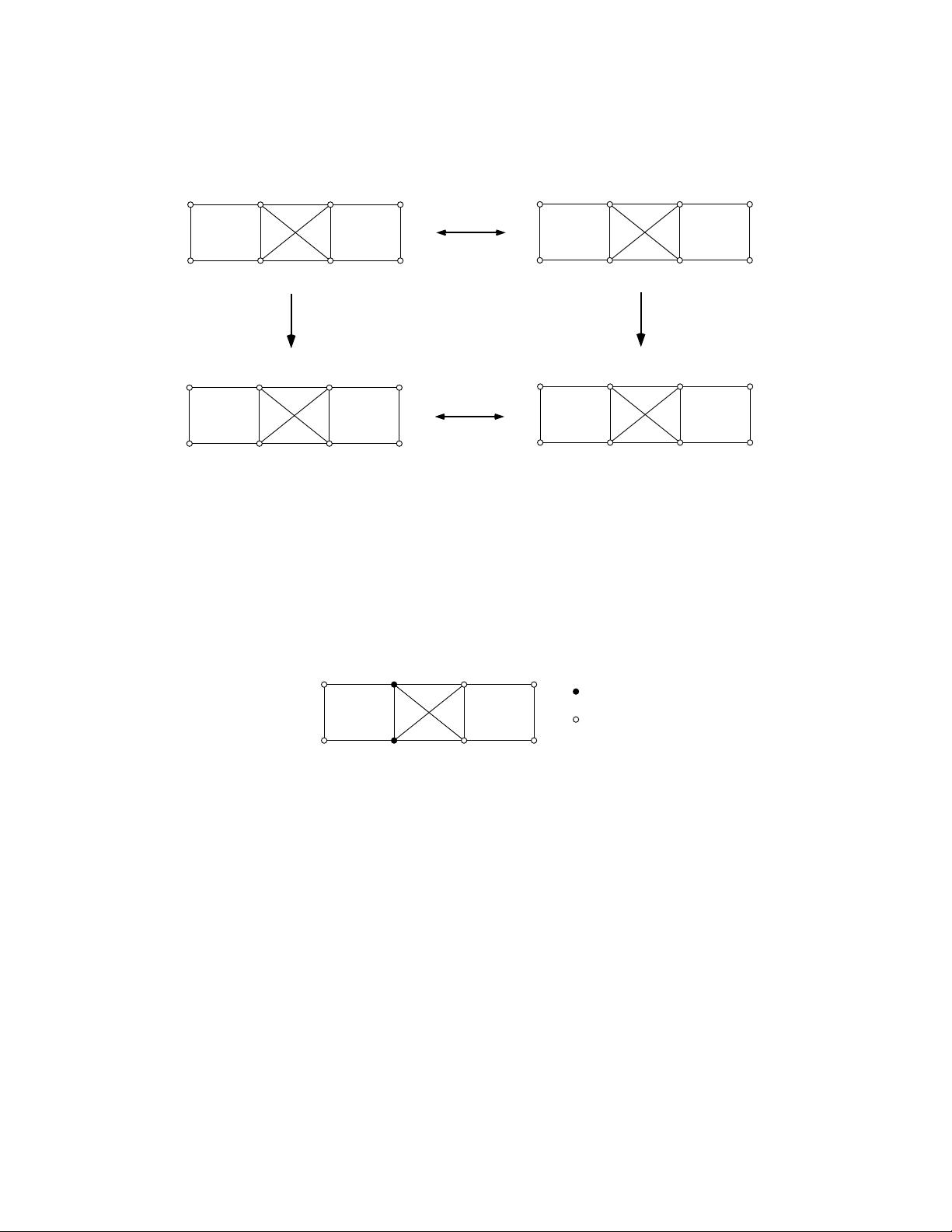
The purpose of canonical labelling is to test isomorphism: two isomorphic graphs
become identical when they are canonically labelled.
Sometimes the vertices of a graph are distinguished from each other according to some
criterion coming from the application. To handle this situation, vertices in nauty and
Traces can be coloured. The definition of “automorphism” respects colours: each vertex
can only be mapped onto a vertex of the same colour. The example below has two vertex
colours, black (•) first and white (◦) second.
second colour
first colour
1
3
2
7
6
0
4
5
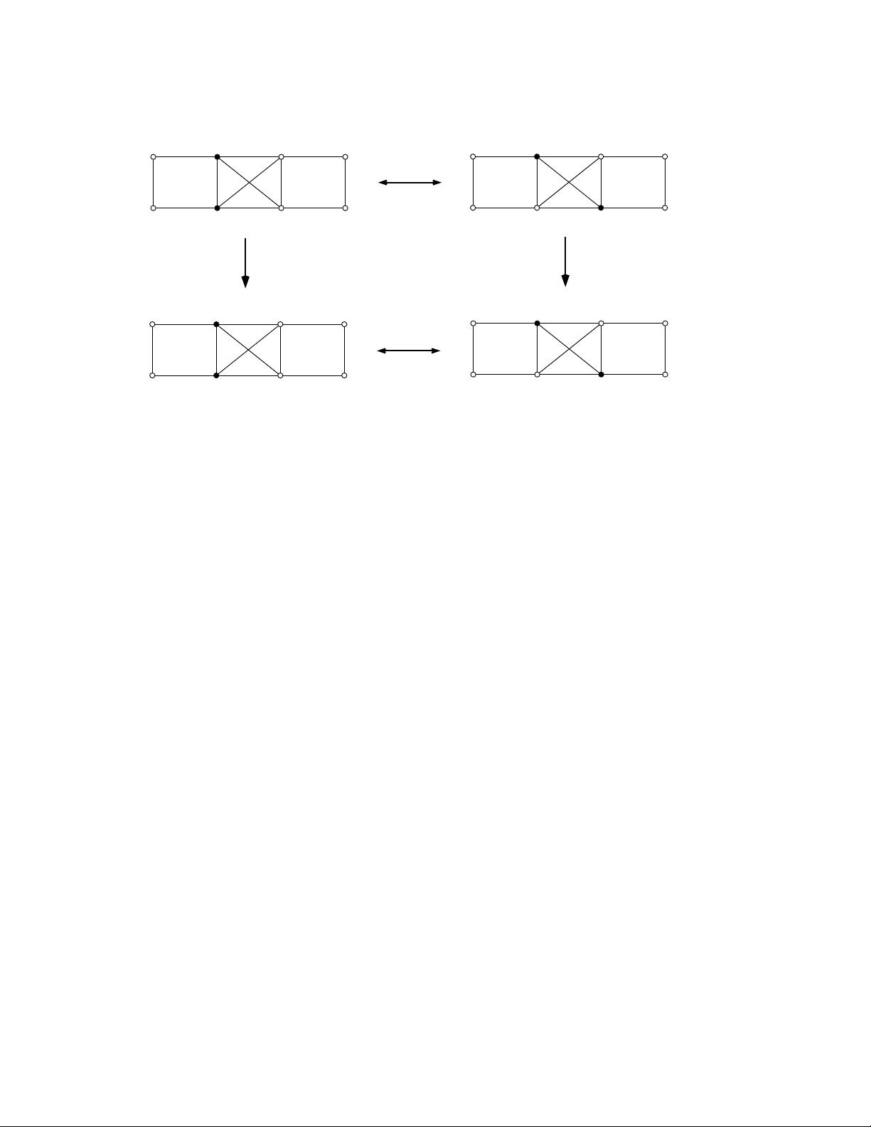
There are now only 4 automorphisms, namely those which preserve the colouring:
(1) (0 1)(2 3)
(4 5)(6 7) (0 1)(2 3)(4 5)(6 7)
nauty and Traces consider the colours to come in some order; i.e., there is a 1st
colour, a 2nd colour, etc.. This doesn’t matter with regard to automorphisms, but it
plays an important part in canonical labelling: the new vertex labels are in order of
colour. The vertices of the first colour are labelled first, of the second colour next, and so
on. This rule means that the canonical labelling can be used to determine if two coloured
graphs are isomorphic via an isomorphism that maps each vertex of one graph onto a
vertex of the same colour in the other graph.
A colouring of the vertices is also referred to as a partition, and the colour classes as
the cells of the partition.
4
different
canonize
different
canonize
0
5
3
6
5 3
1
0
7
6
2
4
6
5
4 0
7
3
2
5
0
7
3
2
4
1
6
1
1
2
7
4
nauty can also handle directed graphs and loops, but Traces currently only handles
simple undirected graphs.
2 dreadnaut
dreadnaut is a simple program which can read graphs and execute nauty or Traces. It
is a rather primitive interface with few facilities.
Input is taken from the standard input and output is sent to the standard output, but
this can be changed by using the “<” and “>” commands. Commands may appear any
number per line separated by white space, commas, semicolons or nothing. They consist
of single characters, except when they consist of two characters. Sometimes commands
are followed by parameters.
At any point of time, dreadnaut knows the following information:
(a) The “mode”, which is one of dense (for using the dense version of nauty; this is
the default), sparse (for using the sparse version of nauty) and Traces (for using
Traces).
(b) The number of vertices, n.
(c) The “current graph” g, if defined.
(d) The “current partition” π. If it is not defined, it is assumed equal to the partition
with every vertex in the same cell (i.e., with the same colour).
(e) The orbits of the (coloured) graph (g, π), if defined.
(f) The canonically labelled isomorph of g, called h, if defined. (Also called canong.)
(g) An extra graph called h
0
, if defined. (Also called savedg.)
(h) Values for each of a variety of options.
In the following ‘#’ is an integer and ‘=’ is always optional.
5


