


17
Chapter 3
Chaotic Signal Generation using a
Blue Diode subject to Optical
Feedback
The goal of the work described in this chapter was to assess the feasibility of using
optical feedback to generate wideband chaotic intensity modulation signals useful for
underwater lidar using recently introduced, commercially available, multimode blue
diode lasers.
3.1 Approach: Exciting Chaotic Intensity Modu-
lation from a Blue Laser Diode using Optical
Feedback
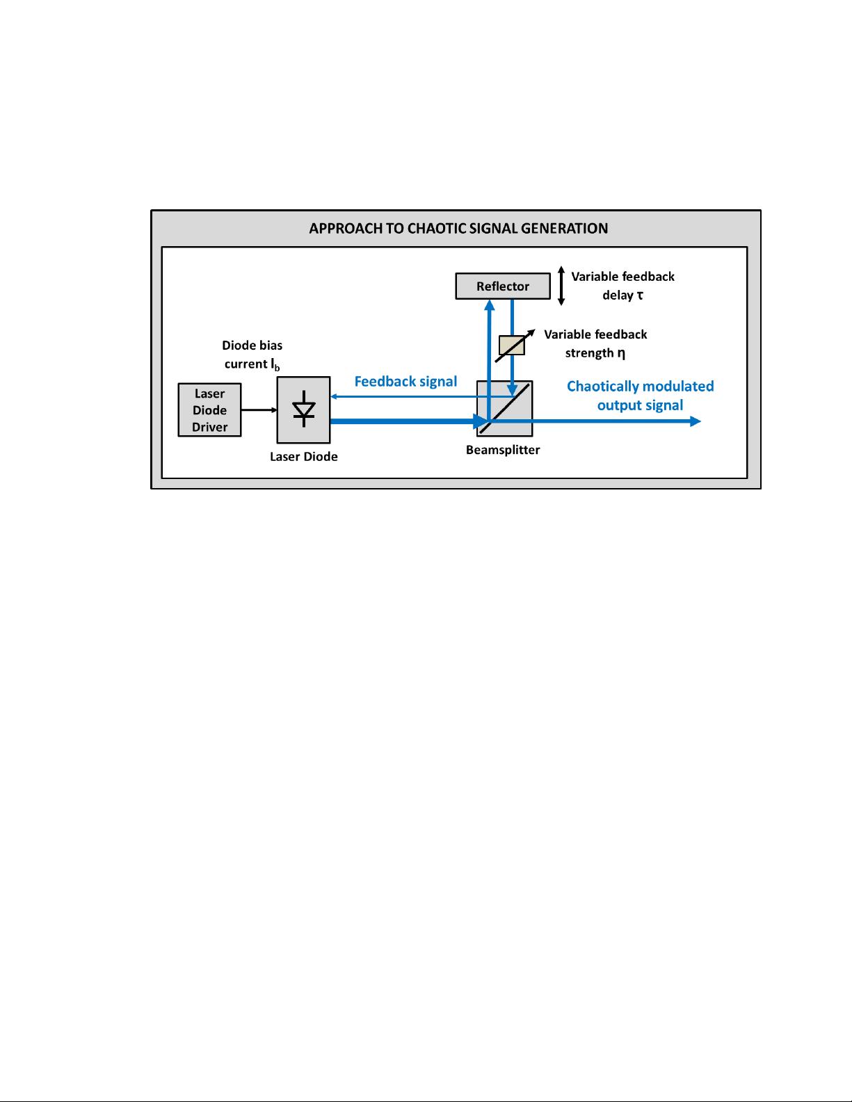
Figure 3.1 shows the optical feedback approach explored for chaotic signal generation.
The proposed approach was to subject a blue semiconductor laser diode to optical
feedback, resulting in a chaotic intensity modulation of the output laser beam. The
18
characteristics of this modulation envelope would then be controlled by varying three
parameters: the laser diode’s bias current I
b
, the feedback strength η, and the feedback
delay τ.
Figure 3.1: Optical feedback approach to chaotic signal generation. A blue laser diode
is subjected to optical feedback, resulting in a chaotically modulated output signal.
The characteristics of this signal are controlled by varying the feedback strength, the
feedback delay, and the laser diode’s bias current.
This approach was investigated using computer and laboratory experiments for
the following tasks:
• Computer experiments:
– Numerically model a multimode diode with optical feedback
– Simulate control over the diode’s intensity modulation output signal; iden-
tify experimental parameters to vary to achieve desirable signals for lidar
• Laboratory experiments:
– Experimentally operate a multimode diode with optical feedback, in a
setup that allows variation of the primary experimental parameters for
signal control

19
– Experimentally validate the signal control trends predicted by the model
– Experimentally generate modulation signals useful for chaotic lidar
As discussed in the previous chapter, the usefulness of an intensity modulated sig-
nal for underwater chaotic lidar was assessed by examining its autocorrelation and
its optical power. Autocorrelations with a narrow main peak and a high peak-to-
sidelobe ratio (PSLR) were considered desirable. These autocorrelation attributes
are associated with non-repeating, wide bandwidth signals, motivating the investi-
gation of wideband noise-like chaotic intensity modulation generation [93–95]. High
modulation depth and high optical power were also desired.
3.2 Computer Experiments
A single multimode diode laser with optical feedback was numerically modeled. The
model was then run for a variety of parameter settings, and the resulting intensity
modulation trends were identified. These insights were used to inform laboratory
experiments by identifying control parameter settings likely to result in desirable
modulation signals.
3.2.1 Numerical Model: A multimode laser diode with opti-
cal feedback
The chaotic signal generation approach shown in Figure 3.1 was modeled using the
Lang-Kobayashi delay-differential equation model for a multimode diode laser sub-
jected to feedback [96], following approach taken by Agrawal’s group in their work on
infrared laser diodes [85]. Equations 3.1-3.6 describe the model. Equation 3.1 models
the electric field in each longitudinal mode E
m
in the laser’s internal waveguide as a
function of time.

20
dE
m
dt
=
1
2
(1 − jα)(G
m
− γ)E
m
(t) + κE
m
(t − τ)e
jωτ
+ ζ
m
+ F
m
(3.1)
Equation 3.2 describes how these longitudinal modes are coupled through the
waveguide’s gain medium, as they compete for the available free carrier electrons N.
dN
dt
=
I
b
q
−
N
τ
e
−
M
X
m=1
G
m
|E
m
(t)|
2
(3.2)
Equations 3.3-3.6 describe calculation of several values needed for Equations 3.1-
3.2. The gain G is calculated from the free carrier population.
G
m
= A(N − N
0
)(1 − (
|m − m
0
|∆ω
L
∆ω
G
)
2
) (3.3)
The mode-interaction term ζ reflects both self- and cross-saturation.
ζ
m
= −
1
2
(β|E
m
|
2
+ θ|E
m
|
2
)E
m
(3.4)
The spontaneous emission noise F is modeled as a Gaussian random variable with
variance based on the cavity loss.
F
m
= N (0, (n
sp
γ)
2
) (3.5)
The feedback coupling coefficient κ is calculated from the internal cavity and the
feedback.
κ =
1 − R
f
τ
L
r
η
R
f
(3.6)
These equations were modeled in Matlab using the dde23.m function [97] and using
the laser parameters listed in Table 3.1. (Full details are available in Appendix A).
These parameters were obtained from literature on laser diodes with feedback [85,98],

21
Table 3.1: Simulation parameters used in computer experiments
Symbol Description Value Units
E
m
Electric field strength in mode m calculated 1
G
m
Gain term for mode m calculated 1/s
N Total free carrier electrons in waveguide calculated 1
F Spontaneous emission noise rate calculated 1
ζ Interaction rate calculated 1/s
κ Feedback coupling coefficient calculated 1
I
b
Laser diode bias current variable C/s
τ Feedback round trip delay time variable s
η Feedback coupling strength variable 1
α Gain parameter 4 1
M Number of spatial modes 7
?
1
R
1
Back facet reflectivity 0.9 1
R
f
Output facet reflectivity 0.12 1
q Electron charge 1.602e-19 C
γ Loss rate 7.26e11 1/s
τ
e
Carrier recombination time 2e9 s
A Gain rate 1.19e3 1/s
N
0
Transparency carrier population 1.64e8 1
τ
L
Internal cavity round trip time 9.3e-12 s
∆ω
G
Material gain width 2π· 1e12 2π· Hz
β Self-saturation rate 4.7e3 1/s
θ Cross-saturation rate 4.4e3 1/s
n
sp
Spontaneous noise magnitude 1.8
?
1
?
Typical values used for predictive simulations are given. Values were changed to M =1,
n
sp
=0 to generate Figures 3.2-3.5 to clarify view of underlying laser dynamics.
not from experimental characterization of in-house lasers. Therefore, the numerical
model provided a qualitative tool for simulating trends in the intensity modulation
signal characteristics as controlled by the bias current and feedback parameters.
In the absence of feedback, the lasing threshold bias current for this simulated laser
was 65 mA; all simulated bias currents should be considered relative to this value.
In the absence of feedback, the relaxation oscillation frequency increased roughly
linearly with bias current, from about 1.1 GHz at threshold to 10 GHz at 500 mA.
All simulated optical feedback delays should be considered relative to the period of
the relaxation oscillation at the selected bias current. (It should be noted that exact


