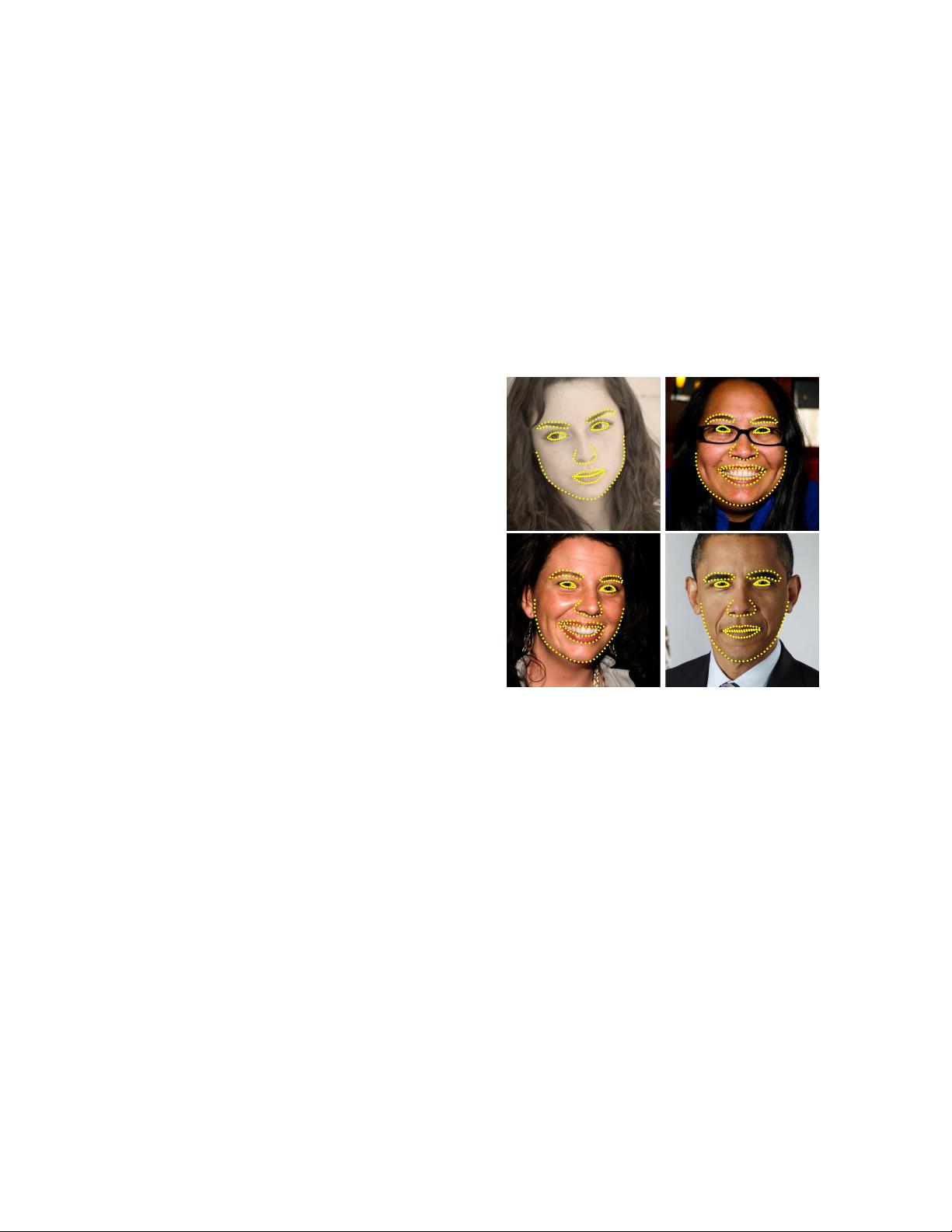
inference/prediction problem. At test time, an alignment al-
gorithm has to estimate the shape, a high dimensional vec-
tor, that best agrees with the image data and our model of
shape. The problem is non-convex with many local optima.
Successful algorithms [4, 9] handle this problem by assum-
ing the estimated shape must lie in a linear subspace, which
can be discovered, for example, by finding the principal
components of the training shapes. This assumption greatly
reduces the number of potential shapes considered during
inference and can help to avoid local optima. Recent work
[8, 11, 2] uses the fact that a certain class of regressors are
guaranteed to produce predictions that lie in a linear sub-
space defined by the training shapes and there is no need
for additional constraints. Crucially, our regression func-
tions have these two elements.
Allied to these two factors is our efficient regression
function learning. We optimize an appropriate loss func-
tion and perform feature selection in a data-driven manner.
In particular, we learn each regressor via gradient boosting
[10] with a squared error loss function, the same loss func-
tion we want to minimize at test time. The sparse pixel set,
used as the regressor’s input, is selected via a combination
of the gradient boosting algorithm and a prior probability on
the distance between pairs of input pixels. The prior distri-
bution allows the boosting algorithm to efficiently explore
a large number of relevant features. The result is a cascade
of regressors that can localize the facial landmarks when
initialized with the mean face pose.
The major contributions of this paper are
1. A novel method for alignment based on ensemble of
regression trees that performs shape invariant feature
selection while minimizing the same loss function dur-
ing training time as we want to minimize at test time.
2. We present a natural extension of our method that han-
dles missing or uncertain labels.
3. Quantitative and qualitative results are presented that
confirm that our method produces high quality predic-
tions while being much more efficient than the best
previous method (Figure 1).
4. The effect of quantity of training data, use of partially
labeled data and synthesized data on quality of predic-
tions are analyzed.
2. Method
This paper presents an algorithm to precisely estimate
the position of facial landmarks in a computationally effi-
cient way. Similar to previous works [8, 2] our proposed
method utilizes a cascade of regressors. In the rest of this
section we describe the details of the form of the individual
components of the cascade and how we perform training.
2.1. The cascade of regressors
To begin we introduce some notation. Let x
i
∈ R
2
be
the x, y-coordinates of the ith facial landmark in an image I.
Then the vector S = (x
T
1
, x
T
2
, . . . , x
T
p
)
T
∈ R
2p
denotes the
coordinates of all the p facial landmarks in I. Frequently,
in this paper we refer to the vector S as the shape. We use
ˆ
S
(t)
to denote our current estimate of S. Each regressor,
r
t
(·, ·), in the cascade predicts an update vector from the
image and
ˆ
S
(t)
that is added to the current shape estimate
ˆ
S
(t)
to improve the estimate:
ˆ
S
(t+1)
=
ˆ
S
(t)
+ r
t
(I,
ˆ
S
(t)
) (1)
The critical point of the cascade is that the regressor r
t
makes its predictions based on features, such as pixel in-
tensity values, computed from I and indexed relative to the
current shape estimate
ˆ
S
(t)
. This introduces some form of
geometric invariance into the process and as the cascade
proceeds one can be more certain that a precise semantic
location on the face is being indexed. Later we describe
how this indexing is performed.
Note that the range of outputs expanded by the ensemble
is ensured to lie in a linear subspace of training data if the
initial estimate
ˆ
S
(0)
belongs to this space. We therefore do
not need to enforce additional constraints on the predictions
which greatly simplifies our method. The initial shape can
simply be chosen as the mean shape of the training data
centered and scaled according to the bounding box output
of a generic face detector.
To train each r
t
we use the gradient tree boosting algo-
rithm with a sum of square error loss as described in [10].
We now give the explicit details of this process.
2.2. Learning each regressor in the cascade
Assume we have training data (I
1
, S
1
), . . . , (I
n
, S
n
)
where each I
i
is a face image and S
i
its shape vector.
To learn the first regression function r
0
in the cascade we
create from our training data triplets of a face image, an
initial shape estimate and the target update step, that is,
(I
π
i
,
ˆ
S
(0)
i
, ∆S
(0)
i
) where
π
i
∈ {1, . . . , n} (2)
ˆ
S
(0)
i
∈ {S
1
, . . . , S
n
}\S
π
i
and (3)
∆S
(0)
i
= S
π
i
−
ˆ
S
(0)
i
(4)
for i = 1, . . . , N. We set the total number of these triplets to
N = nR where R is the number of initializations used per
image I
i
. Each initial shape estimate for an image is sam-
pled uniformly from {S
1
, . . . , S
n
} without replacement.
From this data we learn the regression function r
0
(see
algorithm 1), using gradient tree boosting with a sum of
square error loss. The set of training triplets is then updated


 dlib_face.zip (23个子文件)
  dlib_face
  KazemiCVPR14.pdf 4.81MB
 dlib_face.sln 973B
 Release
  dlib_face.exe 844KB
 dlib_face.pdb 6.39MB
 dlib_face
  2008_007676.jpg 107KB
 dlib_face.vcxproj.filters 950B
 dlib_face.vcxproj.user 165B
 dlib_face.cpp 6KB
 Release
  dlib_face.obj 12.35MB
 vc120.pdb 5.07MB
 dlib_face.log 2KB
 dlib_face.Build.CppClean.log 147B
 dlib_face.tlog
  cl.command.1.tlog 702B
 cl.read.1.tlog 88KB
 link.read.1.tlog 3KB
 link.write.1.tlog 360B
 link.command.1.tlog 1KB
 cl.write.1.tlog 376B
 dlib_face.lastbuildstate 168B
 dlib.lib 23.22MB
 dlib_face.vcxproj 4KB
 dlib_face.sdf 47.81MB
 dlib_face.v12.suo 20KB

 芯光智能2020-01-13官网上的东西
 fhgogo2018-03-17官网上的东西!
 AllyLi02242018-08-13有参考价值
 我的内容管理
展开
 我的资源
快来上传第一个资源
 我的收益 登录查看自己的收益
 我的积分
登录查看自己的积分
 我的C币
登录后查看C币余额
 我的收藏
我的收藏  我的下载
我的下载  下载帮助
下载帮助 
 前往需求广场,查看用户热搜

 信息提交成功
