没有合适的资源?快使用搜索试试~ 我知道了~
关于摄像头自动对焦校准
3星 · 超过75%的资源 需积分: 49 11 下载量 137 浏览量
2015-09-29
09:09:15
上传
评论
收藏 634KB PDF 举报
温馨提示
试读
37页
文献中主要介绍了不同的摄像头校准技术如3D,2D,1D,0D,并且对比了不同校准技术的差异和优点与缺点。
资源推荐
资源详情
资源评论
Chapter 1
CAMERA CALIBRATION
Camera calibration is a necessary step in 3D computer vision in order to extract
metric information from 2D images. It has been studied extensively in computer vi-
sion and photogrammetry, and even recently new techniques have been proposed. In
this chapter, we review the techniques prop osed in the literature include those using
3D apparatus (two or three planes orthogonal to each other, or a plane undergoing
a pure translation, etc.), 2D objects (planar patterns undergoing unknown mo-
tions), 1D objects (wand with dots) and unknown scene points in the environment
(self-calibration). The focus is on presenting these techniques within a consistent
framework.
1.1 Introduction
Camera calibration is a necessary step in 3D computer vision in order to extract
metric information from 2D images. Much work has been done, starting in the
photogrammetry community (see [3, 6] to cite a few), and more recently in computer
vision ([12, 11, 33, 10, 37, 35, 22, 9] to cite a few). According to the dimension of the
calibration objects, we can classify those techniques roughly into three categories.
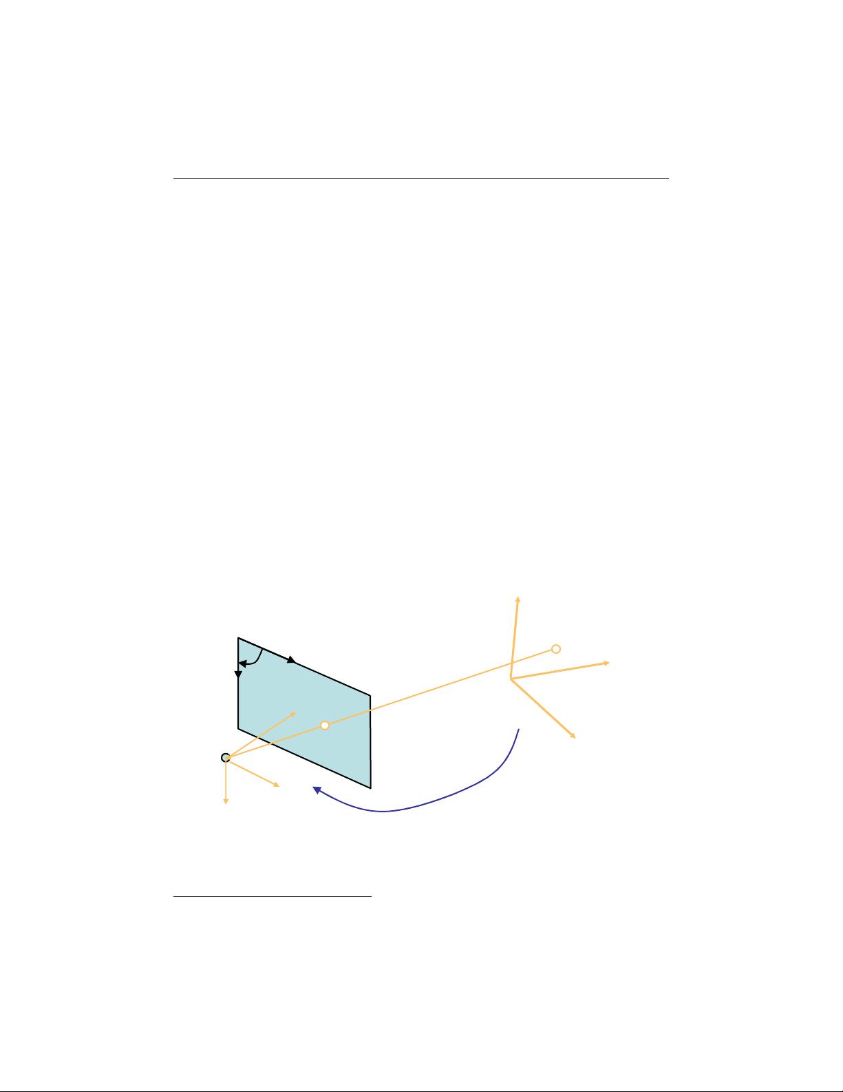
3D reference object based calibration. Camera calibration is performed by ob-
serving a calibration object whose geometry in 3-D space is known with very
good precision. Calibration can be done very efficiently [8]. The calibra-
tion object usually consists of two or three planes orthogonal to each other.
Sometimes, a plane undergoing a precisely known translation is also used [33],
which equivalently provides 3D reference points. This approach requires an
expensive calibration apparatus and an elab orate setup.
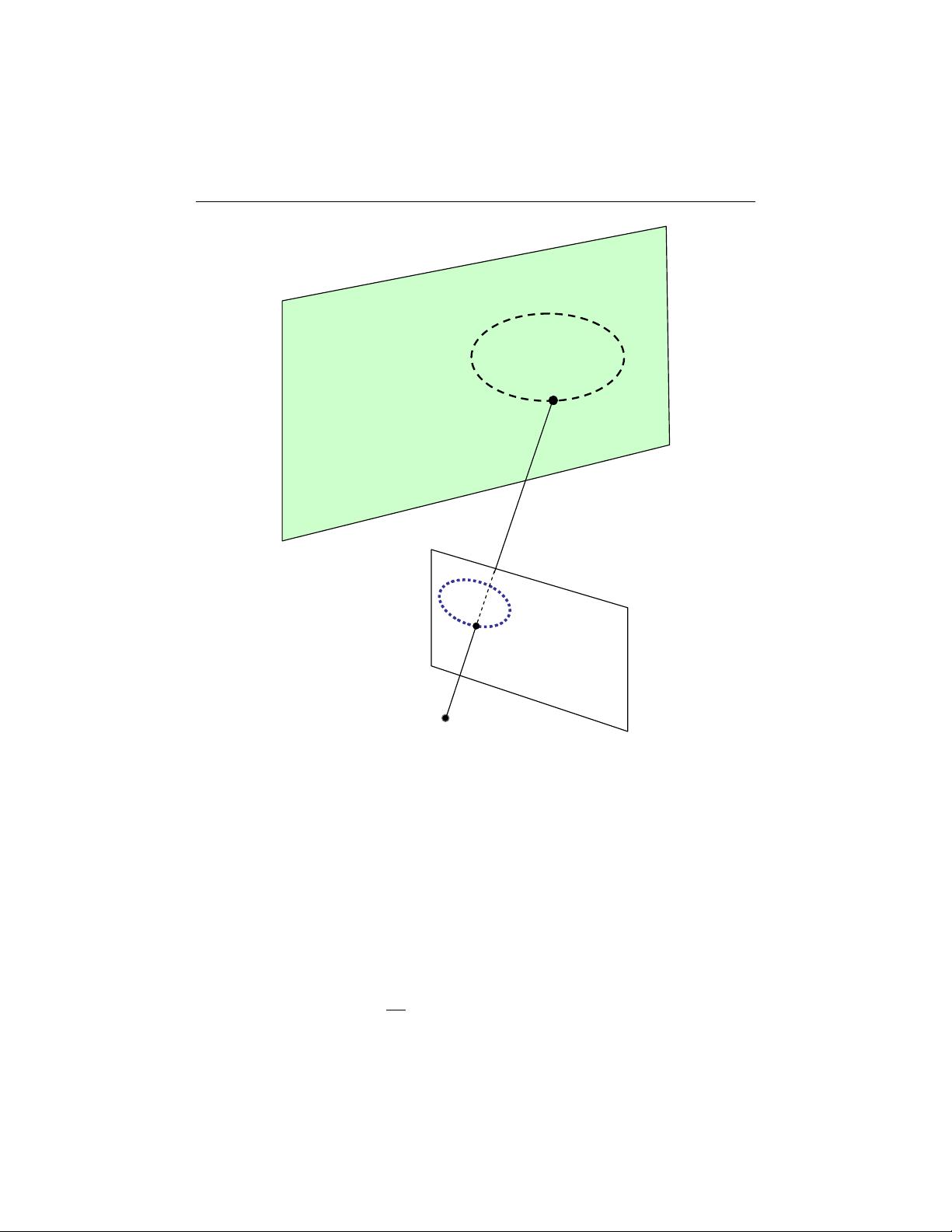
2D plane based calibration. Techniques in this category requires to observe a
planar pattern shown at a few different orientations [42, 31]. Different from
Tsai’s technique [33], the knowledge of the plane motion is not necessary.
Because almost anyone can make such a calibration pattern by him/her-self,
the setup is easier for camera calibration.
1D line based calibration. Calibration objects used in this category are com-
posed of a set of collinear points [44]. As will be shown, a camera can be
1
Z. Zhang, "Camera Calibration", Chapter 2, pages 4-43,
in G. Medioni and S.B. Kang, eds., Emerging Topics in Computer Vision,
Prentice Hall Professional Technical Reference, 2004.
2 Camera Calibration Chapter 1
calibrated by observing a moving line around a fixed point, such as a string
of balls hanging from the ceiling.
Self-calibration. Techniques in this category do not use any calibration object,
and can be considered as 0D approach because only image point correspon-
dences are required. Just by moving a camera in a static scene, the rigidity of
the scene provides in general two constraints [22, 21] on the cameras’ internal
parameters from one camera displacement by using image information alone.
Therefore, if images are taken by the same camera with fixed internal param-
eters, correspondences between three images are sufficient to recover both the
internal and external parameters which allow us to reconstruct 3-D structure
up to a similarity [20, 17]. Although no calibration objects are necessary, a
large number of parameters need to be estimated, resulting in a much harder
mathematical problem.
Other techniques exist: vanishing points for orthogonal directions [4, 19], and cali-
bration from pure rotation [16, 30].
Before going further, I’d like to point out that no single calibration technique
is the b est for all. It really depends on the situation a user needs to deal with.
Following are my few recommendations:
• Calibration with apparatus vs. self-calibration. Whenever possible, if we
can pre-calibrate a camera, we should do it with a calibration apparatus.
Self-calibration cannot usually achieve an accuracy comparable with that of
pre-calibration because self-calibration needs to estimate a large number of
parameters, resulting in a much harder mathematical problem. When pre-
calibration is impossible (e.g., scene reconstruction from an old movie), self-
calibration is the only choice.
• Partial vs. full self-calibration. Partial self-calibration refers to the case where
only a subset of camera intrinsic parameters are to be calibrated. Along the
same line as the previous recommendation, whenever possible, partial self-
calibration is preferred because the number of parameters to be estimated is
smaller. Take an example of 3D reconstruction with a camera with variable
focal length. It is preferable to pre-calibrate the pixel aspect ratio and the
pixel skewness.
• Calibration with 3D vs. 2D apparatus. Highest accuracy can usually be
obtained by using a 3D apparatus, so it should be used when accuracy is
indispensable and when it is affordable to make and use a 3D apparatus. From
the feedback I received from computer vision researchers and practitioners
around the world in the last couple of years, calibration with a 2D apparatus
seems to be the best choice in most situations because of its ease of use and
good accuracy.
• Calibration with 1D apparatus. This technique is relatively new, and it is
hard for the moment to predict how popular it will be. It, however, should be
Section 1.2. Notation and Problem Statement 3
useful especially for calibration of a camera network. To calibrate the relative
geometry between multiple cameras as well as their intrinsic parameters, it
is necessary for all involving cameras to simultaneously observe a number
of points. It is hardly possible to achieve this with 3D or 2D calibration
apparatus
1
if one camera is mounted in the front of a room while another in
the back. This is not a problem for 1D objects. We can for example use a
string of balls hanging from the ceiling.
This chapter is organized as follows. Section 1.2 describes the camera model
and introduces the concept of the absolute conic which is important for camera
calibration. Section 1.3 presents the calibration techniques using a 3D apparatus.
Section 1.4 describes a calibration technique by observing a freely moving planar
pattern (2D object). Its extension for stereo calibration is also addressed. Sec-
tion 1.5 describes a relatively new technique which uses a set of collinear points (1D
object). Section 1.6 briefly introduces the self-calibration approach and provides
references for further reading. Section 1.7 concludes the chapter with a discussion
on recent work in this area.
1.2 Notation and Problem Statement
We start with the notation used in this chapter.
1.2.1 Pinhole Camera Model
C
C
θ
θ
α
β
)
,
(
0
0
v
u
=
Z
Y
X
M
m
m
)
,
(
t
R
Figure 1.1. Pinhole camera model
A 2D point is denoted by m = [u, v]
T
. A 3D point is denoted by M = [X, Y, Z]
T
.
1
An exception is when those apparatus are made transparent; then the cost would be much
higher.
4 Camera Calibration Chapter 1
We use
e
x to denote the augmented vector by adding 1 as the last element:
e
m =
[u, v, 1]
T
and
e
M = [X, Y, Z, 1]
T
. A camera is modeled by the usual pinhole (see
Figure 1.1): The image of a 3D point M, denoted by m is formed by an optical ray
from M passing through the optical center C and intersecting the image plane. The
three points M, m, and C are collinear. In Figure 1.1, for illustration purpose, the
image plane is positioned between the scene point and the optical center, which is
mathematically equivalent to the physical setup under which the image plane is in
the other side with respect to the optical center. The relationship between the 3D
point M and its image projection m is given by
s
e
m = A
£
R t
¤
| {z }
P
e
M ≡ P
e
M , (1.2.1)
with A =
α γ u
0
0 β v
0
0 0 1
(1.2.2)
and P = A
£
R t
¤
(1.2.3)
where s is an arbitrary scale factor, (R, t), called the extrinsic parameters, is the
rotation and translation which relates the world coordinate system to the camera
coordinate system, and A is called the camera intrinsic matrix, with (u
0
, v
0
) the
coordinates of the principal point, α and β the scale factors in image u and v axes,
and γ the parameter describing the skew of the two image axes. The 3 × 4 matrix
P is called the camera projection matrix, which mixes both intrinsic and extrinsic
parameters. In Figure 1.1, the angle between the two image axes is denoted by θ,
and we have γ = α cot θ. If the pixels are rectangular, then θ = 90
◦
and γ = 0.
The task of camera calibration is to determine the parameters of the transfor-
mation b etween an object in 3D space and the 2D image observed by the camera
from visual information (images). The transformation includes
• Extrinsic parameters (sometimes called external parameters): orientation (ro-
tation) and location (translation) of the camera, i.e., (R, t);
• Intrinsic parameters (sometimes called internal parameters): characteristics
of the camera, i.e., (α, β, γ, u
0
, v
0
).
The rotation matrix, although consisting of 9 elements, only has 3 degrees of free-
dom. The translation vector t obviously has 3 parameters. Therefore, there are 6
extrinsic parameters and 5 intrinsic parameters, leading to in total 11 parameters.
We use the abbreviation A
−T
for (A
−1
)
T
or (A
T
)
−1
.
1.2.2 Absolute Conic
Now let us introduce the concept of the absolute conic. For more details, the reader
is referred to [7, 15].
Section 1.2. Notation and Problem Statement 5
0
1
=
∞
−−
∞
mAAm
TT
C
∞
m
∞
x
Absolute Conic
0=
∞∞
xx
T
Image of
Absolute Conic
Figure 1.2. Absolute conic and its image
A point x in 3D space has projective coordinates
e
x = [x
1
, x
2
, x
3
, x
4
]
T
. The
equation of the plane at infinity, Π
∞
, is x
4
= 0. The absolute conic Ω is defined by
a set of points satisfying the equation
x
2
1
+ x
2
2
+ x
2
3
= 0
x
4
= 0 .
(1.2.4)
Let x
∞
= [x
1
, x
2
, x
3
]
T
be a point on the absolute conic (see Figure 1.2). By
definition, we have x
T
∞
x
∞
= 0. We also have
e
x
∞
= [x
1
, x
2
, x
3
, 0]
T
and
e
x
T
∞
e
x
∞
= 0.
This can be interpreted as a conic of purely imaginary points on Π
∞
. Indeed, let
x = x
1
/x
3
and y = x
2
/x
3
be a point on the conic, then x
2
+ y
2
= −1, which is an
imaginary circle of radius
√
−1.
An important property of the absolute conic is its invariance to any rigid trans-
剩余36页未读,继续阅读
资源评论
- 镁锌2017-03-22不是Autofocus校准,是张氏标定
jolin_
- 粉丝: 0
- 资源: 1
上传资源 快速赚钱
- 我的内容管理 展开
- 我的资源 快来上传第一个资源
- 我的收益 登录查看自己的收益
- 我的积分 登录查看自己的积分
- 我的C币 登录后查看C币余额
- 我的收藏
- 我的下载
- 下载帮助
安全验证
文档复制为VIP权益,开通VIP直接复制
信息提交成功