没有合适的资源?快使用搜索试试~ 我知道了~
资源推荐
资源详情
资源评论
©ARTVILLE
[
Ivan W. Selesnick, Richard G. Baraniuk, and Nick G. Kingsbury
]
The Dual-Tree Complex
Wavelet Transform
[
A coherent framework
for multiscale signal and
image processing
]
T
he dual-tree complex wavelet transform (
C
WT) is a relatively
recent enhancement to the discrete wavelet transform (DWT),
with important additional properties: It is nearly shift invariant
and directionally selective in two and higher dimensions. It
achieves this with a redundancy factor of only
2
d
for
d
-dimen-
sional signals, which is substantially lower than the undecimated DWT. The
multidimensional (M-D) dual-tree
C
WT is nonseparable but is based on a
computationally efficient, separable filter bank (FB). This tutorial discusses
the theory behind the dual-tree transform, shows how complex wavelets with
good properties can be designed, and illustrates a range of applications in sig-
nal and image processing. We use the complex number symbol
C
in
C
WT to
1053-5888/05/$20.00©2005IEEE IEEE SIGNAL PROCESSING MAGAZINE [123] NOVEMBER 2005
Authorized licensed use limited to: HUNAN UNIVERSITY. Downloaded on May 21,2010 at 04:33:20 UTC from IEEE Xplore. Restrictions apply.
IEEE SIGNAL PROCESSING MAGAZINE [124] NOVEMBER 2005
avoid confusion with the often-used acronym CWT for the (dif-
ferent) continuous wavelet transform.
BACKGROUND
This article aims to reach two different audiences. The first is the
wavelet community, many members of which are unfamiliar
with the utility, convenience, and unique properties of complex
wavelets. The second is the broader class of signal processing folk
who work with applications where the DWT has proven some-
what disappointing, such as those involving complex or modulat-
ed signals (radar, speech, and music, for example) or higher-
dimensional, geometric data (geophysics and imaging, for exam-
ple). In these problems, the complex wavelets can potentially
offer significant performance improvements over the DWT.
THE WAVELET TRANSFORM
AND MULTISCALE ANALYSIS
Since its emergence 20 years ago, the wavelet transform has
been exploited with great success across the gamut of signal
processing applications, in the process, often redefining the
state-of-the-art performance [102], [112]. In a nutshell, the
DWT replaces the infinitely oscillating sinusoidal basis functions
of the Fourier transform with a set of locally oscillating basis
functions called wavelets. In the classical setting, the wavelets
are stretched and shifted versions of a fundamental, real-valued
bandpass wavelet
ψ(t)
. When carefully chosen and combined
with shifts of a real-valued low-pass scaling function
φ(t)
, they
form an orthonormal basis expansion for one-dimensional (1-D)
real-valued continuous-time signals [27]. That is, any finite-
energy analog signal
x(t)
can be decomposed in terms of
wavelets and scaling functions via
x(t) =
∞
n=−∞
c(n)φ(t − n)
+
∞
j =0
∞
n =−∞
d( j, n) 2
j/2
ψ(2
j
t − n). (1)
The scaling coefficients
c(n)
and wavelet coefficients
d( j, n)
are
computed via the inner products
c(n) =
∞
−∞
x(t)φ(t − n) dt,(2)
d( j, n) = 2
j/2
∞
−∞
x(t)ψ(2
j
t − n) dt.(3)
They provide a time-frequency analysis of the signal by measur-
ing its frequency content (controlled by the scale factor
j
) at dif-
ferent times (controlled by the time shift
n
).
There exists a very efficient, linear time complexity algorithm
to compute the coefficients
c(n)
and
d( j, n)
from a fine-scale rep-
resentation of the signal (often simply
N
samples) and vice versa
based on two octave-band, discrete-time FBs that recursively
apply a discrete-time low-pass filter
h
0
(n)
, a high-pass filter
h
1
(n)
, and upsampling and downsampling operations (see Figure
24) [27], [69]. These filters provide a convenient parameterization
for designing wavelets and scaling functions with desirable prop-
erties, such as compact time support and fast frequency decay (to
ensure the analysis is as local as possible in time frequency) and
orthogonality to low-order polynomials (vanishing moments)
[27]. See “Real-Valued Discrete Wavelet Transform and Filter
Banks” for more background on wavelets, FBs, and their design.
Why have wavelets and multiscale analysis proved so useful
in such a wide range of applications? The primary reason is
[FIG1] In the neighborhood of an edge, the real DWT produces
both large and small wavelet coefficients. In contrast, the
(approximately) analytic
C
WT produces coefficients whose
magnitudes are more directly related to their proximity to the
edge. Here, the test signal is a step edge at
n = n
o
,
x(n) = u(n −n
o
)
. The figure shows the value of the wavelet
coefficient
d(0, 8)
(the eighth coefficient at stage 3 in “Real-
Valued Discrete Wavelet Transform and Filter Banks,” Figure 24)
as a function of
n
o
. In the top panel, the real coefficient
d(0, 8)
is
computed using the conventional real DWT. In the lower panel,
the complex coefficient
d(0, 8)
is computed using the dual-tree
C
WT. (The filters used here are the same as those in Figure 2.)
20 40 60 80 100 120
0
0.5
1
Value of d(0,8), Real Wavelet Transform
n
o
20 40 60 80 100 120
0
0.1
0.2
0.3
0.4
0.5
0.6
0.7
|d(0,8)|, Dual-Tree Complex Wavelet Transform
n
o
Authorized licensed use limited to: HUNAN UNIVERSITY. Downloaded on May 21,2010 at 04:33:20 UTC from IEEE Xplore. Restrictions apply.
IEEE SIGNAL PROCESSING MAGAZINE [125] NOVEMBER 2005
because they provide an
extremely efficient rep-
resentation for many
types of signals that
appear often in practice
but are not well matched
by the Fourier basis,
which is ideally meant
for periodic signals. In
particular, wavelets pro-
vide an optimal repre-
sentation for many
signals containing sin-
gularities (jumps and
spikes), the archetypal
example being a piece-
wise smooth function
consisting of low-order
polynomials separated
by jump discontinuities.
The wavelet representa-
tion is optimally sparse
for such signals, requir-
ing an order of magni-
tude fewer coefficients
than the Fourier basis to
approximate within the
same error. The key to
the sparsity is that since
wavelets oscillate locally,
only wavelets overlap-
ping a singularity have
large wavelet coeffi-
cients; all other coeffi-
cients are small.
The sparsity of the
wavelet coefficients of
many real-world signals
enables near-optimal sig-
nal processing based on simple thresholding (keep the large coef-
ficients and kill the small ones), the core of a host of powerful
image compression (JPEG2000 [98]), denoising, approximation,
and deterministic and statistical signal and image algorithms.
TROUBLE IN PARADISE: FOUR PROBLEMS
WITH REAL WAVELETS
However, this is not the end of the story. In spite of its efficient com-
putational algorithm and sparse representation, the wavelet trans-
form suffers from four fundamental, intertwined shortcomings.
PROBLEM 1: OSCILLATIONS
Since wavelets are bandpass functions, the wavelet coefficients tend
to oscillate positive and negative around singularities (see Figures 1
and 2). This considerably complicates wavelet-based processing,
making singularity extraction and signal modeling, in particular,
very challenging [22]. Moreover, since an oscillating function passes
often through zero, we see that the conventional wisdom that sin-
gularities yield large wavelet coefficients is overstated. Indeed, as we
see in Figure 1, it is quite possible for a wavelet overlapping a singu-
larity to have a small or even zero wavelet coefficient.
PROBLEM 2: SHIFT VARIANCE
A small shift of the signal greatly perturbs the wavelet coeffi-
cient oscillation pattern around singularities (see Figure 2).
Shift variance also complicates wavelet-domain processing;
algorithms must be made capable of coping with the wide range
of possible wavelet coefficient patterns caused by shifted singu-
larities [34], [55], [59], [80], [83].
To better understand wavelet coefficient oscillations and shift
variance, consider a piecewise smooth signal
x(t − t
0
)
like the
step function
[FIG2] The wavelet coefficients of a signal
x(n)
are very sensitive to translations of the signal. For two
impulse signals
x(n) = δ(n − 60)
and
x(n) = δ(n − 64)
(a), we plot the wavelet coefficients
d(j, n)
at a
fixed scale
j
(b) and (c). (b) shows the real coefficients computed using the conventional real discrete
wavelet transform (DWT, with Daubechies length-14 filters). (c) shows the magnitude of the complex
coefficients computed using the dual-tree complex discrete wavelet transform (
C
WT with length-14 filters
from [58]). For the dual-tree
C
WT the total energy at scale
j
is nearly constant, in contrast to the real DWT.
0 50 100
0
0.2
0.4
0.6
0.8
1
Test Signal x(n) = δ (n–60)
0 5 10 15
−0.2
−0.1
0
0.1
0.2
0.3
d(0,n), Real DWT, Energy = 0.046226
0 5 10 15 20
0
0.05
0.1
0.15
0.2
0.25
0.3
0.35
|d(0,n)|, Complex WT, Energy = 0.12365
0 50 100
0
0.2
0.4
0.6
0.8
1
Test Signal x(n) = δ(n–64)
0 5 10 15
−0.2
−0.1
0
0.1
0.2
0.3
d(0,n), Real DWT, Energy = 0.084775
0 5 10 15 20
0
0.05
0.1
0.15
0.2
0.25
0.3
0.35
|d(0,n)|, Complex WT, Energy = 0.12377
Authorized licensed use limited to: HUNAN UNIVERSITY. Downloaded on May 21,2010 at 04:33:20 UTC from IEEE Xplore. Restrictions apply.
IEEE SIGNAL PROCESSING MAGAZINE [126] NOVEMBER 2005
u(t) =
0 t < 0
1 t ≥ 0
analyzed by a wavelet basis having a sufficient number of van-
ishing moments. Its wavelet coefficients consist of samples of
the step response of the wavelet [80], [83]
d( j, n) ≈ 2
−3 j/2
2
j
t
0
−n
−∞
ψ(t) dt,
where
is the height of the jump. Since
ψ(t)
is a bandpass
function that oscillates around zero, so does its step response
d( j, n)
as a function of
n
(recall Figure 1). Moreover, the factor
2
j
in the upper limit (
j ≥ 0
) amplifies the sensitivity of
d( j, n)
to the time shift
t
0
, leading to strong shift variance.
PROBLEM 3: ALIASING
The wide spacing of the wavelet coefficient samples, or equivalent-
ly, the fact that the wavelet coefficients are computed via iterated
discrete-time downsampling operations interspersed with nonideal
low-pass and high-pass filters, results in substantial aliasing. The
inverse DWT cancels this aliasing, of course, but only if the wavelet
and scaling coefficients are not changed. Any wavelet coefficient
processing (thresholding, filtering, and quantization) upsets the
delicate balance between the forward and inverse transforms, lead-
ing to artifacts in the reconstructed signal.
PROBLEM 4: LACK OF DIRECTIONALITY
Finally, while Fourier sinusoids in higher dimensions correspond
to highly directional plane waves, the standard tensor product
construction of M-D wavelets produces a checkerboard pattern
that is simultaneously oriented along several directions. This
lack of directional selectivity greatly complicates modeling and
processing of geometric image features like ridges and edges.
ONE SOLUTION: COMPLEX WAVELETS
Fortunately, there is a simple solution to these four DWT short-
comings. The key is to note that the Fourier transform does not
suffer from these problems. First, the
magnitude of the Fourier transform
does not oscillate positive and negative
but rather provides a smooth positive
envelope in the Fourier domain.
Second, the magnitude of the Fourier
transform is perfectly shift invariant,
with a simple linear phase offset
encoding the shift. Third, the Fourier
coefficients are not aliased and do not
rely on a complicated aliasing cancel-
lation property to reconstruct the sig-
nal; and fourth, the sinusoids of the
M-D Fourier basis are highly direc-
tional plane waves.
What is the difference? Unlike the
DWT, which is based on real-valued oscillating wavelets, the
Fourier transform is based on complex-valued oscillating sinusoids
e
jt
= cos(t ) + j sin(t)(4)
with
j =
√
−1
. The oscillating cosine and sine components (the
real and imaginary parts, respectively) form a Hilbert transform
pair; i.e., they are
90
◦
out of phase with each other. Together
they constitute an analytic signal
e
jt
that is supported on only
one-half of the frequency axis (
>0
). See “The Hilbert
Transform and Analytic Signal” for more background.
Inspired by the Fourier representation, imagine a
C
WT as
in (1)–(3) but with a complex-valued scaling function and
complex-valued wavelet
ψ
c
(t ) = ψ
r
(t ) + j ψ
i
(t ).
Here, by analogy to (4),
ψ
r
(t )
is real and even and
jψ
i
(t )
is
imaginary and odd. Moreover, if
ψ
r
(t )
and
ψ
i
(t )
form a Hilbert
transform pair (
90
◦
out of phase with each other), then
ψ
c
(t )
is
an analytic signal and supported on only one-half of the fre-
quency axis. The complex scaling function is defined similarly.
See Figure 3 for an example of a complex wavelet pair that
approximately satisfies these properties.
Projecting the signal onto
2
j/2
ψ
c
(2
j
t − n)
as in (3), we
obtain the complex wavelet coefficient
d
c
( j, n) = d
r
( j, n) + j d
i
( j, n)
with magnitude
|d
c
( j, n)|=
[d
r
( j, n)]
2
+ [d
i
( j, n)]
2
and phase
d
c
( j, n) = arctan
d
i
( j, n)
d
r
( j, n)
[FIG3] A q-shift complex wavelet corresponding to a set of orthonormal dual-tree filters of
length 14 [58].
0 2 4 6 8 10 12
−1.5
−1
−0.5
0
0.5
1
1.5
2
t
ψ
h
(t), ψ
g
(t)
Wavelets
−8 −6 −4 −2 0 2 4 6 8
0
0.5
1
1.5
2
ω/π
|Ψ
h
(ω) + j Ψ
g
(ω)|
Frequency Spectrum
Authorized licensed use limited to: HUNAN UNIVERSITY. Downloaded on May 21,2010 at 04:33:20 UTC from IEEE Xplore. Restrictions apply.
IEEE SIGNAL PROCESSING MAGAZINE [127] NOVEMBER 2005
when
|d
c
( j, n)| > 0
. As with the Fourier transform, complex
wavelets can be used to analyze and represent both real-
valued signals (resulting in symmetries in the coefficients)
and complex-valued signals. In either case, the
C
WT enables
new coherent multiscale signal processing algorithms that
exploit the complex magnitude and phase. In particular, as we
will see, a large magnitude indicates the presence of a singu-
larity while the phase indicates its position within the support
of the wavelet [81], [83], [113], [117].
The theory and practice of discrete complex wavelets can be
broadly classed into two schools. The first seeks a
ψ
c
(t )
that
forms an orthonormal or biorthogonal basis [9], [11], [37], [64],
[108], [114]. As we show below, this strong constraint prevents
the resulting
C
WT from overcoming most of the four DWT
shortcomings outlined above. The second school seeks a redun-
dant representation, with both
ψ
r
(t )
and
ψ
i
(t )
individually
forming orthonormal or biorthogonal bases. The resulting
C
WT
is a
2×
redundant tight frame [26] in 1-D, with the power to
overcome the four shortcomings.
In this article, we will focus on a particularly natural
approach to the second, redundant type of
C
WT, the dual-
tree approach, which is based on two FB trees and thus two
bases [55], [57]. As we will see, any
C
WT based on wavelets
of compact support cannot exactly possess the Hilbert
transform/analytic signal properties, and this means that
any such
C
WT will not perfectly overcome the four DWT
shortcomings. The key challenge in dual-tree wavelet design
is thus the joint design of its two FBs to yield a complex
wavelet and scaling function that are as close as possible to
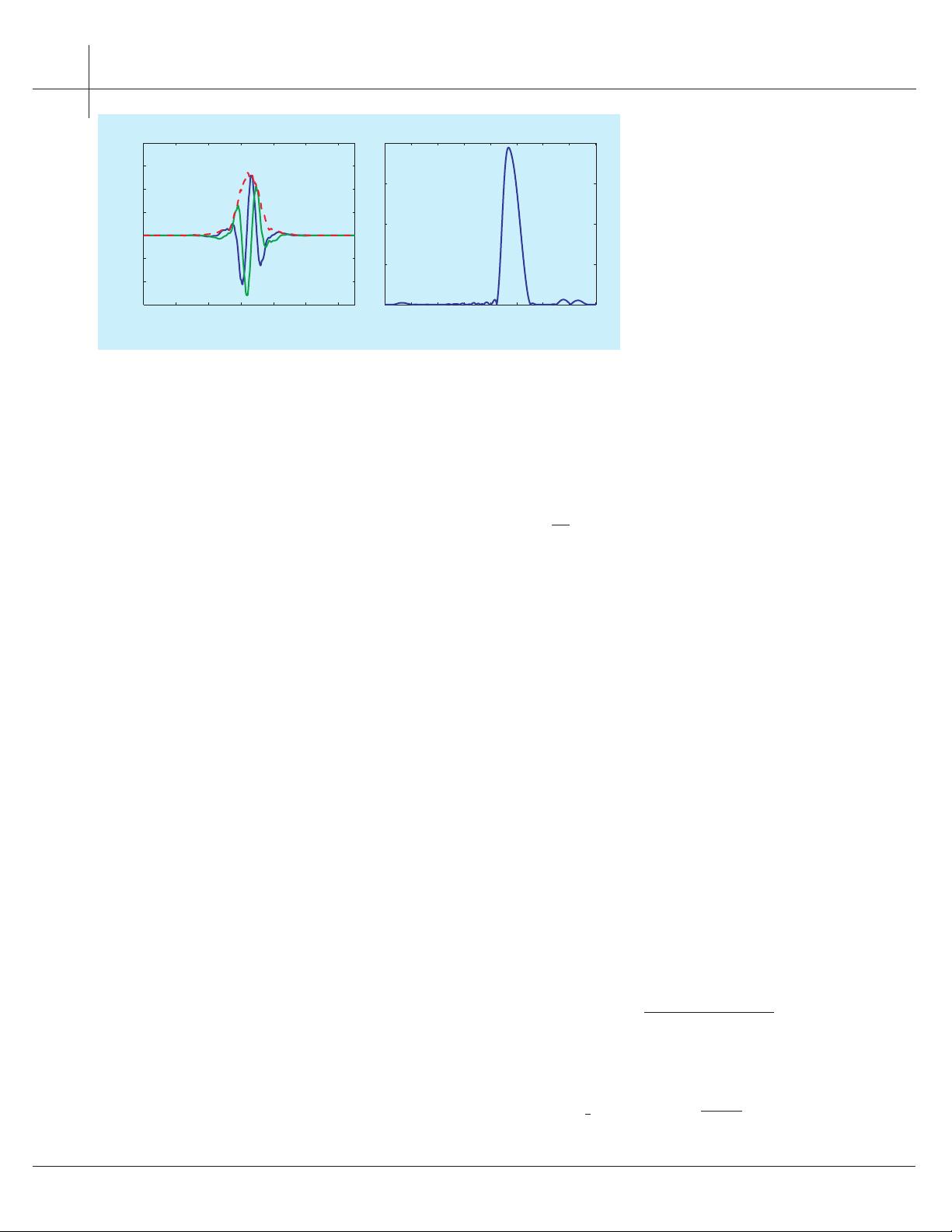
analytic. From Figure 3, we see that we can reach quite close
to the ideal even with quite short filters.
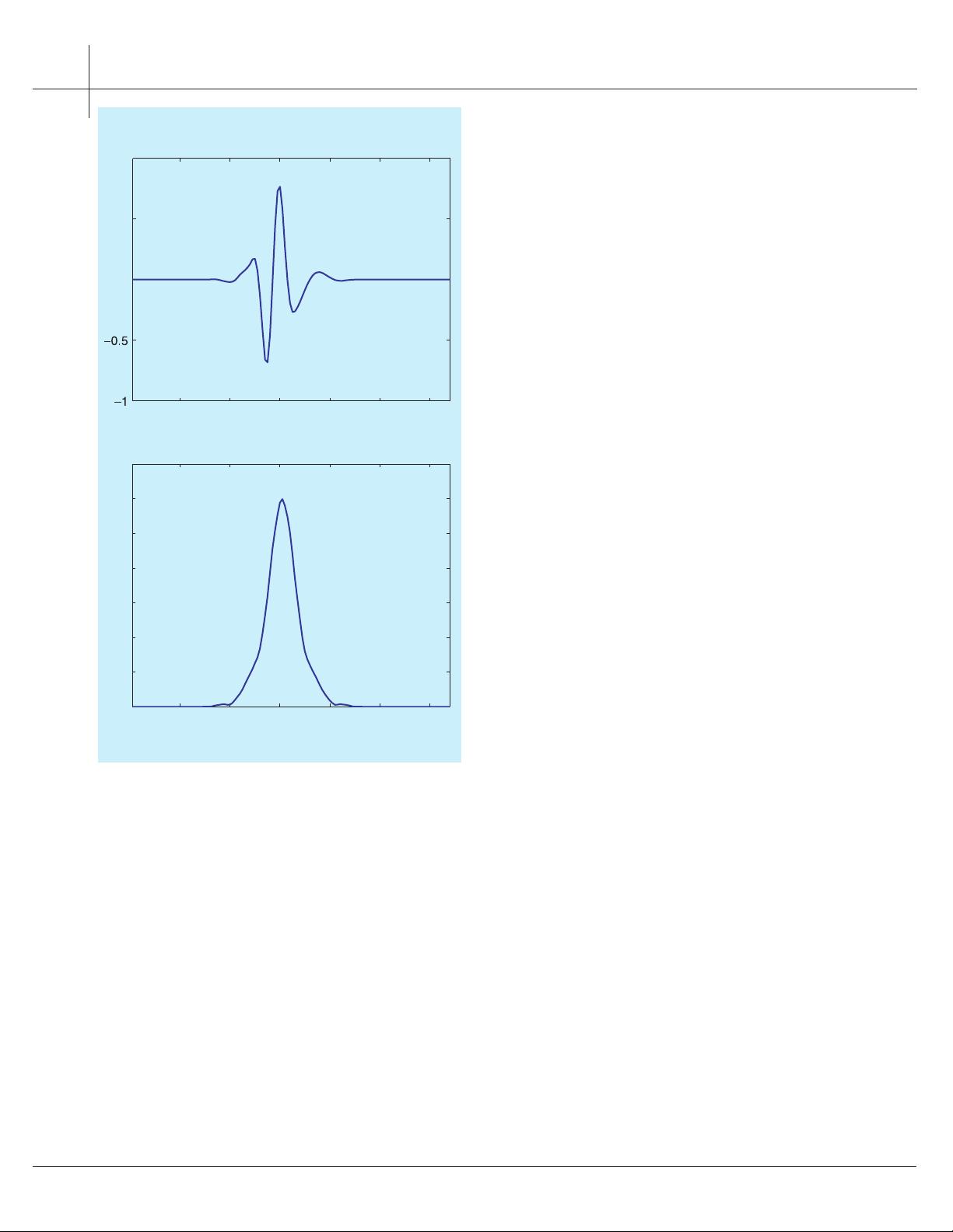
As a result, the dual-tree
C
WT comes very close to mirror-
ing the attractive properties of the Fourier transform, includ-
ing a smooth, nonoscillating magnitude (see Figure 1); a
nearly shift-invariant magnitude with a simple near-linear
phase encoding of signal shifts; substantially reduced aliasing;
and directional wavelets in higher dimensions. The only cost
for all of this is a moderate redundancy:
2×
redundancy in 1-D
(
2
d
for
d
-dimensional signals, in general). This is much less
than the
log
2
N×
redundancy of a perfectly shift-invariant
DWT [22], [63], which, moreover, will not offer the desirable
magnitude/phase interpretation of the
C
WT nor the good
directional properties in higher dimensions.
COMPLEX WAVELET COMPLEXITIES
The design of complex analytic wavelets raises several unique
and nontrivial challenges that do not arise with the real DWT. In
this section, we overview them and discuss a straightforward but
limited approach to the
C
WT that provides a jumping off point
for the dual-tree.
ANALYTICITY VERSUS FINITE SUPPORT
It is often desired in wavelet-based signal processing that the
wavelet be well localized in time. (In many applications, the
wavelet
ψ(t)
will actually have finite support.) Finitely sup-
ported wavelets are of special interest because, in this case,
the DWT can be easily implemented with finite impulse
response (FIR) filters. However, a finitely supported function
can never be exactly analytic, because the Fourier transform
of a finitely supported function can never be exactly zero on
an interval
[A, B]
with
B > A
(on any set of positive measure
to be exact) let alone on the entire positive or negative fre-
quency axis [77]. Thus, any exactly analytic wavelet must have
infinite support (and slow decay, in fact).
Thus, if we want finitely supported wavelets, then we must
accept wavelets that are only approximately analytic and a
C
WT
that is only approximately magnitude/phase, shift invariant, and
free from aliasing. We can relax the finite support condition, but
the resulting infinitely supported wavelets are beyond the scope
of this article. The design challenge will be to see how close we
can get to analyticity. Unfortunately, the standard approach to
designing and implementing wavelet transforms (with FIR or
infinite impulse response (IIR) filters) has basic limitations even
for approximately analytic wavelets, as we now illustrate.
ANALYTICITY VERSUS PERFECT RECONSTRUCTION
The question of how to design filters
h
0
(n)
and
h
1
(n)
satisfying
the perfect reconstruction (PR) conditions so that the wavelet
ψ(t)
has short support and vanishing moments was answered
by Daubechies [25]. Note, however, that Daubechies’ wavelets
are not analytic. Can we design the filters
h
i
(n)
in Figure 24
such that the corresponding scaling function and wavelet given
by (60) and (59) are complex and (approximately) analytic?
While complex filters satisfying the PR conditions have been
developed [11], [42], [64], [123], those solutions do not give ana-
lytic wavelets and do not have the desirable properties of analyt-
ic wavelets described previously. (They do, however, have
desirable symmetry properties.) It turns out that the design of a
complex (approximately) analytic wavelet basis is more difficult
than the design of a real wavelet basis. If we follow the standard
approach for wavelet design, then problems arise when we
require the wavelet to be analytic.
So that the dyadic dilations and translations of a single func-
tion
ψ(t)
(the wavelet) constitute a basis for signal expansion,
ψ(t)
must satisfy certain constraints. Unfortunately, these con-
straints make it difficult to design a wavelet
ψ(t)
that is also
analytic. Specifically, analytic solutions are not possible because
the PR conditions (see “Real-Valued Discrete Transform and
Filter Banks”) require that
H
0
e
j ω
H
0
e
j ω
+ H
1
e
j ω
H
1
e
j ω
= 2
for
−π ≤ ω ≤ π.
Suppose that
h
1
(n)
is (approximately) ana-
lytic. Then
H
1
(e
j ω
) ≈ 0
for
−π<ω<0,
which in turn
implies that
H
0
(e
j ω
)
H
0
(e
j ω
) ≈ 2
for
−π<ω<0.
That is, nei-
ther
H
0
(z)
nor
H
0
(z)
is a reasonable low-pass filter and, conse-
quently, the dilation equation does not have a well-defined
solution. Therefore, the wavelet corresponding to the usual
DWT cannot be approximately analytic.
Authorized licensed use limited to: HUNAN UNIVERSITY. Downloaded on May 21,2010 at 04:33:20 UTC from IEEE Xplore. Restrictions apply.
剩余28页未读,继续阅读
资源评论
- wk198702052012-06-06文章对双树复值小波的学习非常有帮助,感谢分享。
- eishra2011-10-11很好,是原版,谢谢了
- chengfy032017-06-04很好用,值得推荐
zy7880815
- 粉丝: 6
- 资源: 5
上传资源 快速赚钱
- 我的内容管理 展开
- 我的资源 快来上传第一个资源
- 我的收益 登录查看自己的收益
- 我的积分 登录查看自己的积分
- 我的C币 登录后查看C币余额
- 我的收藏
- 我的下载
- 下载帮助
安全验证
文档复制为VIP权益,开通VIP直接复制
信息提交成功