AdeepbeliefnetworkwithPLSRfornonlinearsystemmodeling资源-CSDN文库

研究论文

64 浏览量 2021-02-07 09:40:15 上传评论收藏 902KB PDF 举报

资源推荐

资源详情

资源评论

Neural Networks 104 (2018) 68–79

Contents lists available at ScienceDirect

Neural Networks

journal homepage: www.elsevier.com/locate/neunet

A deep belief network with PLSR for nonlinear system modeling

Junfei Qiao

a,b,

*, Gongming Wang

a,b

, Wenjing Li

a,b

, Xiaoli Li

Faculty of Information Technology, Beijing University of Technology, Beijing 100124, China

Beijing Key Laboratory of Computational Intelligence and Intelligent System, Beijing 100124, China

a r t i c l e i n f o

Article history:

Received 16 April 2017

Received in revised form 5 October 2017

Accepted 17 October 2017

Available online 31 October 2017

Keywords:

Deep belief network

Partial least square regression

Weights optimization

Nonlinear system modeling

Wastewater treatment system

a b s t r a c t

Nonlinear system modeling plays an important role in practical engineering, and deep learning-based

deep belief network (DBN) is now popular in nonlinear system modeling and identification because of

the strong learning ability. However, the existing weights optimization for DBN is based on gradient,

which always leads to a local optimum and a poor training result. In this paper, a DBN with partial least

square regression (PLSR-DBN) is proposed for nonlinear system modeling, which focuses on the problem

of weights optimization for DBN using PLSR. Firstly, unsupervised contrastive divergence (CD) algorithm is

used in weights initialization. Secondly, initial weights derived from CD algorithm are optimized through

layer-by-layer PLSR modeling from top layer to bottom layer. Instead of gradient method, PLSR-DBN can

determine the optimal weights using several PLSR models, so that a better performance of PLSR-DBN

is achieved. Then, the analysis of convergence is theoretically given to guarantee the effectiveness of

the proposed PLSR-DBN model. Finally, the proposed PLSR-DBN is tested on two benchmark nonlinear

systems and an actual wastewater treatment system as well as a handwritten digit recognition (nonlinear

mapping and modeling) with high-dimension input data. The experiment results show that the proposed

PLSR-DBN has better performances of time and accuracy on nonlinear system modeling than that of other

methods.

1. Introduction

In the past several years, systems modeling has achieved great

progress because of great demands for controller design (Jia, Li,

& Wang, 2016; Martensson & Hjalmarsson, 2011; Qiao & Han,

2012), process analysis (Zhang, Chai, & Li, 2012) and soft computing

(Han, Chen, & Qiao, 2011; Han & Qiao, 2013). However, most

practical systems are nonlinear, especially industrial systems, and

the dynamic behavior of the systems cannot be described using a

linear model. In fact, it is difficult to model nonlinear systems due

to the existence of uncertainty, including structure and parameters

(Gandomi & Alavi, 2011). Therefore, nonlinear system modeling is

a significant and challenging work (Anderson & Kadirkamanathan,

2007), which has been attracting a lot of attention in many fields.

Theoretically, ANNs can approximate any nonlinear system to

any accuracy (Leung, Lam, & Ling, 2003; Scarselli & Tsoi, 1998).

As a result, ANNs have been widely used for nonlinear systems

modeling (Han, Wang, & Qiao, 2013; Li, Qiao, & Han, 2016). For

example, a self-organizing cascade neural network (SCNN) with

random weight is proposed for nonlinear system modeling (Li et al.,

Corresponding author at: Faculty of Information Technology, Beijing University

of Technology, Beijing 100124, China.

E-mail addresses: junfeiq@bjut.edu.cn (J. Qiao), xiaowangqsd@163.com

(G. Wang), wenjing.li@bjut.edu.cn (W. Li), lixiaolibjut@bjut.edu.cn (X. Li).

2016), and the modeling accuracy is improved to some extent. An

adaptive second order algorithm (ASOA) is developed to train the

fuzzy neural network (FNN) to achieve fast and robust convergence

for nonlinear system modeling (Han, Ge, & Qiao, 2016), and the

corresponding results are satisfactory. A hierarchical radial basis

function (HRBF) neural network is proposed for nonlinear system

modeling in wastewater treatment process (Han & Qiao, 2013), and

the corresponding performances of modeling and prediction are

both acceptable for the practical system. However, these methods

mentioned above only consider the single hidden layer architec-

ture, resulting in the lack of significant improvements for modeling

accuracy. From universal approximation theory, if the number of

hidden neurons is enough and even equal to the number of training

samples, a single hidden layer neural network can approximate

any nonlinear systems to any desired accuracy (Huang, Chen,

& Siew, 2006; Leung et al., 2003). However, a neural network

with the number of hidden neurons equal to training samples is

impractical, especially under the condition of numerous training

samples. Therefore, how to solve this contradictory problem is still

challenging for improving accuracy of nonlinear systems modeling.

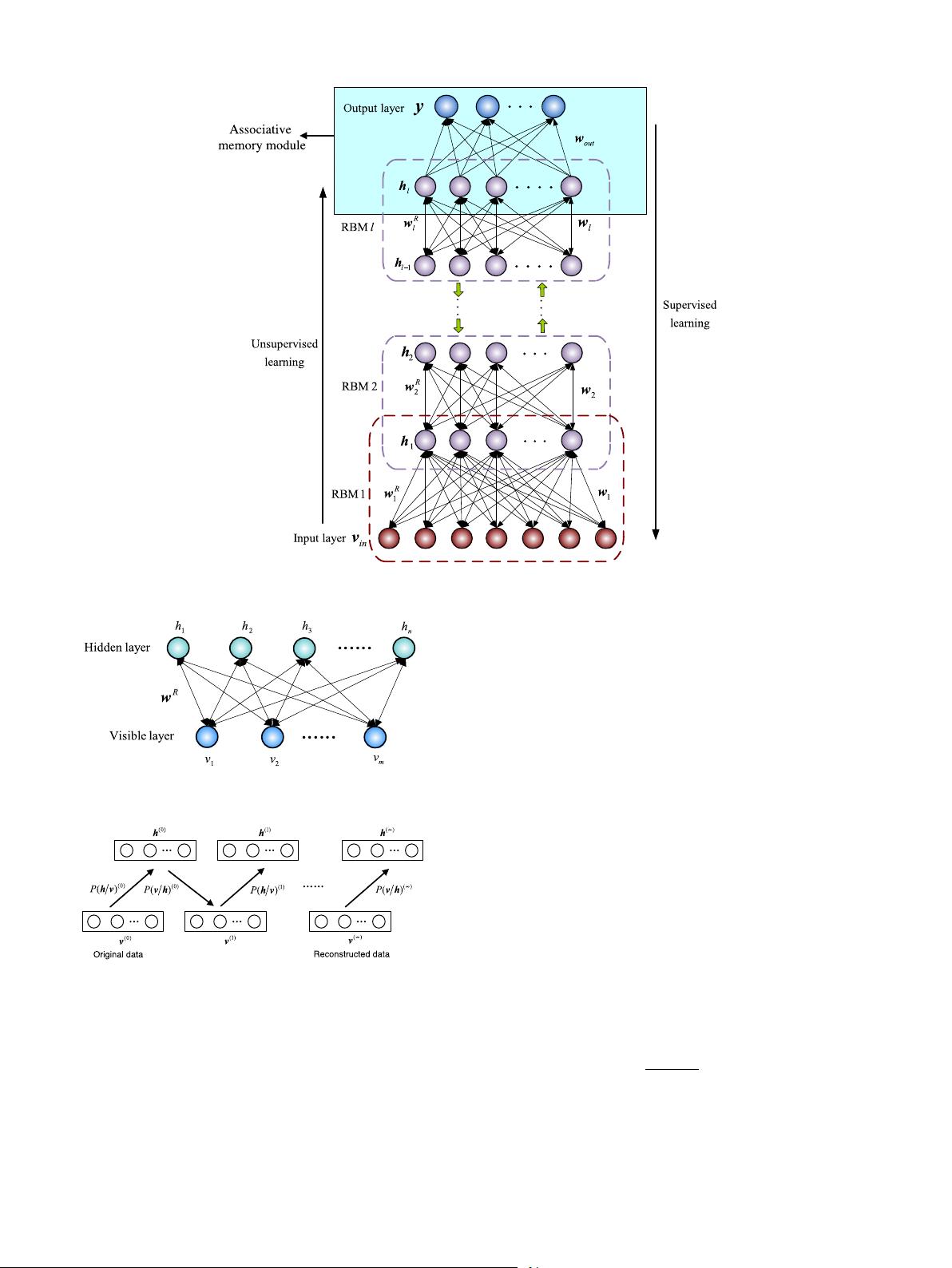
Recently, researches show that deep learning-based deep belief

network (DBN) can achieve any desired modeling accuracy with

less hidden neurons (Hinton, Osindero, & Teh, 2006; Rosa & Yu,

2016). DBN is a kind of neural network with a deep architecture

(several hidden layers), which features hierarchical representation

https://doi.org/10.1016/j.neunet.2017.10.006

J. Qiao et al. / Neural Networks 104 (2018) 68–79 69

inspired by biological neural systems (Hinton & Salakhutdinov,

2006; LeCun, Bengio, & Hinton, 2015). DBN is composed of several

restricted Boltzmann Machines (RBMs) stacked sequentially, and

the output of the front RBM is treated as the input of the following

RBM. The learning process of DBN includes two sections: unsuper-

vised learning and supervised learning. Unsupervised learning is

implemented by contrastive divergence (CD) algorithm to initialize

the weights of DBN (Bengio & Senécal, 2008), which is superior to

random weight initialization in ANNs (Bengio, Courville, & Vincent,

2013). Supervised learning is to fine-tune the initial weight derived

from unsupervised learning using error-propagation algorithm.

Because of the efficient learning capability of extracting features

from samples data, DBN has begun to be applied to nonlinear sys-

tem modeling (Shen, Chao, & Zhao, 2015). However, the supervised

learning of DBN is a gradient-based algorithm starting from the

top layer (target output) to the bottom layer (input layer). This is

always time-consuming and easily leads to local minimum even

training failure (Eom, Jung, & Sirisena, 2003; Horikawa, Furuhashi,

& Uchikawa, 1992; Jagannathan & Lewis, 1996), especially when it

comes to DBN with too many hidden layers. It needs to be pointed

that local minimum is an enormous threat to learning capability,

which leads to a lower accuracy of DBN for nonlinear system

modeling.

To overcome the above difficulties, it is necessary to find a

learning method without gradient. Partial least square regression

(PLSR), as a layer-to-layer linear regression model, focuses on

searching the global minimum without gradient. The training sam-

ples used in PLSR are directly collected from the supervised data

of the input layer and the output layer. The problems of modeling

and prediction have been researched in literatures (He, Geng, & Xu,

2015; Janik, Forrester, & Rawson, 2009), where the weight between

the input layer and output layer is optimized by PLSR model, and

the performances for modeling and prediction are correspondingly

improved. Therefore, the PLSR-based supervised learning scheme

can significantly improve the modeling accuracy and shortens the

learning time as well. It has been demonstrated that the neural net-

works combined with PLSR-based method can achieve a feasible

and satisfactory performance for nonlinear systems modeling and

identification (He et al., 2015; Janik et al., 2009). Unfortunately,

the existing neural networks combined with PLSR-based method

have only considered the single-hidden-layer architecture, which

weakens the superiority of combination with PLSR-based method.

To avoid the problems resulted from gradient-based algorithm

and achieve a better modeling accuracy, a DBN with PLSR (PLSR-

DBN) is proposed for nonlinear systems modeling in this paper.

This proposed PLSR-DBN replaces the gradient-based algorithm

using PLSR in supervised learning, which can avoid these problems

resulted from gradient-based algorithm and achieve a better mod-

eling accuracy. Firstly, unsupervised CD algorithm is conducted

to initialize weight of PLSR-DBN using samples data, and the ob-

tained initial weight is used to extract features from samples data.

Once the initial weight is determined, the features of all hidden

layers calculated by the initial weight are correspondingly frozen.

Secondly, PLSR algorithm is used to optimize the initial weight

from the top layer to the bottom layer. Particularly, PLSR model

is constructed in every two layers starting from the top layer, and

the training data of the top layer and the other hidden layers are

collected from the target output and the frozen features. Finally,

the proposed PLSR-DBN is tested on nonlinear dynamic system

modeling, Lorenz chaotic time series prediction and total phospho-

rus prediction in a practical wastewater treatment process as well

as handwritten digit recognition with high-dimension input data.

The structure of this paper is organized as follows. Section 2

gives a brief overview of DBN. The details of the proposed PLSR-

DBN algorithm are given in Section 3, including the architecture

and learning process as well as convergence analysis. Section 4

presents the experimental results and discussions, which demon-

strates the performance of the proposed PLSR-DBN compared with

other existing similar methods. Finally, the conclusions of this

work are given in Section 5.

2. Deep belief network

DBN is composed of several RBMs stacked sequentially, and

RBM is the primary element of DBN. The learning process of DBN

can be divided into two stages: unsupervised learning and su-

pervised learning. Firstly, unsupervised learning is implemented

by CD algorithm, which trains the stacked RBMs to obtain the

initial weights W



, w

l−1

, . . . , w



. Secondly, supervised

learning is always implemented by error back-propagation (BP)

algorithm, which fine-tunes the initial weight to obtain the final

weight W = (w

out

, w

l−1

, . . . , w

, w

). Particularly, the top

two layers are defined as the joint distribution of the last hidden

layer (h

) and the output layer (desired output), which is called

as associative memory module. It should be pointed out that, the

existing supervised learning (BP algorithm) of DBN is conducted

from the associative memory module to input layer. The basic

architecture of DBN is shown in Fig. 1, and l is the number of hidden

layers.

2.1. Unsupervised learning

The main purpose of unsupervised learning is to determine the

initial weights only using input samples, which is implemented

by training the RBMs stacked sequentially. The architecture of

RBM is shown in Fig. 2, where v =

(

, v

, . . . , v

)

and h =

(

, h

, . . . , h

)

denote the state of the visible layer and hidden

layer respectively, and w

is a m × n weight matrix connecting

the visible and hidden neurons. Given the parameters set θ =

, a, b}, the joint probability distribution P (v, h; θ) and energy

function E (v, h; θ) are described as

P(v, h; θ) =

−E(v,h;θ)

(1)

E(v, h; θ) = −



i=1

−



j=1

−



i=1



j=1

(2)

where Z =



v, h

−E(v, h; θ)

is the partition function, w

is the

connecting weight of RBM, and a

and b

are the biases of the

visible neuron and the hidden neuron respectively. The marginal

probability distribution with respect to v is described as

P(v; θ) =



−E(v,h;θ)

. (3)

It is necessary to calculate the derivative of P (v; θ) with respect to

, and the weight can be updated as follows.

∆w

∂ log P(v; θ)

∂w

= E

data

) − E

model

) (4)

= w

+ η∆w

(5)

where η is learning rate, E

data

) is the expectation of observed

data in training set, and E

model

) is the expectation of sampling

data in model. Usually, it is very difficult to compute E

model

so Gibbs sampling (Bengio et al., 2013) is used to approximately

compute E

model

). The process of Gibbs sampling is shown in

Fig. 3.

During the process of Gibbs sample, conditional probability

distributions of visible neurons and hidden neurons are described

剩余11页未读，继续阅读

评论收藏

内容反馈

weixin_38614825

粉丝: 6
资源: 951

A deep belief network with PLSR for nonlinear system modeling

1.2 Deep Belief Network(DBN)(Milestone of Deep Learning Eve).rar

Deep Belief Network深度信念网络（DBN的Matlab代码）

DeeBNetV3.2.zip_Deep Belief_deep belief network_deep learning_de

A fast learning algorithm for deep belief nets

深层信念网络.rar_deep belief network_深层信念网络

A fast learning algorithm for deep belief nets.rar

A Fast Learning Algorithm for Deep Belief Nets

《A fast learning algorithm for deep belief nets》原文

深度学习--深度信念网络(Deep-Belief-Network)

deep belief network toolbox written in Matlab

Deep Belief Network_DBN_RBM_matlab源码

Deep Belief Nets in C++ and CUDA C_Volume 1-Apress(2018)

Deep Belief Network in Matlab_DBN_RBM_matlab源码

Deep Belief Nets in C++ and CUDA C Volume 2

Deep-Belief-Network-for-Regression-master.zip_deep belief networ

An Algorithm for Bayesian Belief Network Construction from Data

Simple tutotial code for Deep Belief Network (DBN).zip

行人惯性导航零速检测算法

基于CORDIC的反正弦和反余弦计算的FPGA实现

混合动力汽车基于规则的控制和ECMS与优化等效因子的实时能源管理策略

使用3DCNN和卷积LSTM进行手势识别学习时空特征

BA无标度网络中的SIR模型

基于三次贝塞尔曲线的类汽车曲率连续路径平滑

基于机器学习的设备剩余寿命预测方法综述

基于开源工具集的大数据网络安全态势感知及预警架构

基于无差拍预测控制和扰动观测器的永磁同步电机电流控制

基于FPGA的奇异值和特征值分解的快速实现。

基于BP神经网络的人口预测

无人机协同目标的多无人机协同搜索方法

最新资源