没有合适的资源?快使用搜索试试~ 我知道了~
learning from data 下半部
4星 · 超过85%的资源 需积分: 10 87 下载量 31 浏览量
2016-05-31
14:38:46
上传
评论 1
收藏 15.06MB PDF 举报
温馨提示
试读
203页
Yaser S. Abu-Mostafa 教授所著的机器学习教材下半部。 非影印,非常清晰。 是 caltech 《learning from data》和台大林轩田教授《机器学习基石》的指定教材。 主要讲授机器学习的理论问题。算是介绍学习理论比较浅显易懂的入门教材了。
资源推荐
资源详情
资源评论
e-
CHAPTER
e-Chapter 6
Similarity-Based Methods
“It’s a manohorse”, exclaimed the confident little 5
year old boy. We call it the Centaur out of habit, but
who can fault the kid’s intuition? The 5 year old has
never seen this thing before now, yet he came up with
a reasonable classification for the beast. He is using
the simplest method of learning that we know of –
similarity – and yet it’s effective: the child searches
through his history for similar objects (in this cas e a
man and a horse) and builds a classification ba sed on
these similar objects.
The method is simple and intuitive, yet when we
get into the details, several issues need to be addressed
in order to arrive at a technique that is quantitative
and fit for a computer. The goal of this chapter is to build ex actly such a
quantitative framework for similarity based learning.
6.1 Simila ri ty
The “manohorse” is interesting because it requires a deep understanding of
similarity: first, to say that the Centaur is similar to both man and horse;
and, second, to decide that there is enough similarity to both objects so that
neither can be excluded, warranting a new class. A good measure of similarity
allows us to not only classify objects using similar objects, but also detect the
arrival of a new class of objects (novelty detection).
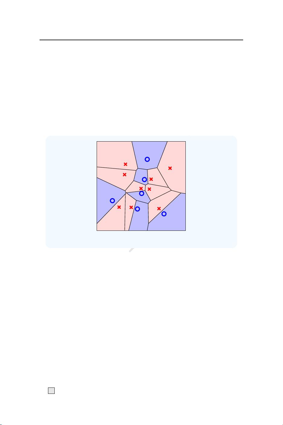
A simple classification rule is to give a new input the class of the most
similar input in your data. This is the “nea rest neighbor” rule. To implement
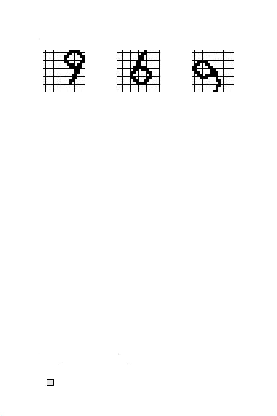
the nearest neighbor rule, we need to first qua ntify the similar ity between
two objects. There are different ways to measure similarity, or equivalently
dissimilarity. Consider the following example with 3 digits.
c
A
M
L
Yaser Abu-Mostafa, Malik Magdon-Ismail, Hsuan-Tien Lin: Oct-2014.
All rights reserved. No commercial use or re-distribution in any format.
e-
CHAPTER
e-6. Similarity-Based Methods 6.1. Similarity
The two 9s should be regarded as very similar. Yet, if we naively measure
similarity by the number of black pixels in common, the two 9s have only two
in c ommon. On the other hand, the 6 has many more black pixels in common
with either 9, even though the 6 should be regarded as dissimilar to both 9s.
Before measuring the similarity, one should prepr oces s the inputs, for example
by centering, axis aligning and normalizing the size in the case of an image.
One can go further and extract the relevant features of the data, for example
size (number of black pixels) and symmetry as was done in Chapter 3. These
practical consider ations regarding the natur e of the learning task, though im-
portant, are not our primary focus here. We will assume that through domain
expertise or otherwise, features have been co ns tructed to identify the impor-
tant dimensions, and if two inputs differ in these dimensions, then the inputs
are likely to be dissimilar. Given this assumption, there are well established
ways to measure similarity (or dissimilarity) in different contexts.
6.1.1 Similarity Measures
For inputs x, x
′
which are vectors in R
d
, we can measure dissimilarity using
the standard Euclidean distance,
d(x, x
′
) = kx −x
′
k.
The smaller the distance, the more similar are the objects corresponding to
inputs x and x
′
. For Boolean feature s the Euclidean distance is the square
root of the well known Hamming distance. The Euclidean distance is a sp e c ial
case of a more general distance measure which can be defined for an arbitrary
positive semi-definite matrix Q:
d(x, x
′
) = (x −x
′
)
t
Q(x − x
′
).
A useful special case, known as the Mahalanobis distance is to set Q = Σ
−1
,
where Σ is the covar iance matrix
1
of the data. The Mahalanobis distance
metric depends on the data set. The ma in advantage of the Ma halanobis
distance over the standard Euclidean distance is tha t it takes into account
correla tions among the data dimensions and scale. A similar effect can be
accomplished by first using input preprocess ing to standardize the data (see
1
Σ =
1
N
N
X
i=1
x
i
x
t
i
−
¯
x
¯
x
t
, where
¯
x =
1
N
N
X
i=1
x
i
.
c
A
M
L
Abu-Mostafa, Magdon-Ismail, Lin: Oct-2014 e-Chap:6–2
e-
CHAPTER
e-6. Similarity-Based Methods 6.2. Nearest Neighbor
Chapter 9) and then using the standard Euclidean distance. Ano ther useful
measure, espec ially for Boolean vectors, is the cosine similarity,
CosSim(x, x
′
) =
x
•
x
′
kxkkx
′
k
.
The cosine similarity is the cosine of the angle between the two vectors,
CosSim ∈ [−1, 1], and larger values indica te greater similarity. When the
objects represent sets, then the set similarity or Jaccard coefficient is often
used. For example, consider two movies which have be e n watched by two dif-
ferent sets of users S
1
, S
2
. We may measure how similar these movies are by
how similar the two sets S
1
and S
2
are:
J(S
1
, S
2
) =
|S
1
∩ S
2
|
|S
1
∪ S
2
|
;
1 −J(S
1
, S
2
) can be used as a measure of distance which conveniently has the
properties that a metric formally satisfies, such as the tr iangle inequality. We
fo c us on the Euclidean distance which is als o a metric; many of the algo rithms,
however, apply to arbitrary similarity measures.
Exercise 6.1
(a) Give two vectors with very high cosine similarity but very low Euclidean
distance similarity. Similarly, give two vectors with very low cosine
similarity but very high Euclidean distance similarity.
(b) If we shift the origin of the coordinate system, which of the two
measures of similarity will change? How will this affect your choice
of features?
6.2 Nearest Neighbo r
Simple rules survive; and, the nearest neighbor technique is perhaps the sim-
plest of all. We will summarize the entire algorithm in a short paragraph.
But, before we forge ahead, let’s not forget the two basic competing principles
laid out in Part I: any lear ning technique should be expressive enough that
we can fit the data and obtain low E
in
; however, it should be reliable enough
that a low E
in
implies a low E
out
.
The nearest neighbor rule is embarrassingly simple. There is no training
phase (or no “learning” so to speak ). The entire algor ithm is sp e c ified by how
one computes the final hypo thesis g(x) on a test input x. Reca ll that the data
set is D = (x
1
, y
1
) . . . (x
N
, y
N
), where y
n
= ±1. To clas sify the test point x,
find the nearest point to x in the data s et (the nearest neighbor), and use the
classification of this nearest neighbor.
Fo rmally speaking, reorder the data according to distance from x (breaking
ties using the data point’s index for simplicity). We wr ite (x
[n]
(x), y
[n]
(x))
c
A
M
L
Abu-Mostafa, Magdon-Ismail, Lin: Oct-2014 e-Chap:6–3
e-
CHAPTER
e-6. Similarity-Based Methods 6.2. Nearest Neighbor
for the nth such reordered data point with res pect to x. We will drop the
dependence on x and s imply write (x
[n]
, y
[n]
) when the context is clear. So,
d(x, x
[1]
) ≤ d(x, x
[2]
) ≤ ··· ≤ d(x, x
[N]
)
The final hypothesis is
g(x) = y
[1]
(x)
(x is classified by just looking at the class of the near e st data point to x). This
simple nearest neighbor rule admits a nice geometric interpretation, shown for
two dimensions in Figure 6.1.
Figure 6.1: Nearest neighbor Voronoi tessellation.
The shading illustrates the final hypothesis g(x). Each data point x
n
‘owns’ a
region of the space defined by the set of points clo ser to x
n
than to any other
data point. These regions are co nvex polytopes (convex regions whose faces
are hyperplanes), some of which are unb ounded; in two dimensions, we get
convex polygons . The resulting set of regions defined by such a set of points is
called a Voronoi (or Dirichlet) tessellation of the space. The final hypothesis g
is a Voronoi tessellation with each region inheriting the class of the data point
that owns the region. Figure 6.2(a) shows the nea rest neighbor c lassifier for a
sample of 500 data points from the digits data described in Chapter 3 (blue
circles are the digit 1 and all other digits are the red x’s).
The clear advantage of the nearest neighbor rule is that it is embarrass-
ingly simple and intuitive, easy to implement and there is no training. It is
expressive, as it achieves zero in sample er ror (as ca n immediately be deduced
from Figure 6.1), and as we will soon see, it is reliable. A practically important
cosmetic upside, when (for example) presenting to a client, is that the classi-
fication of a test object is e asy to ‘explain’: just present the similar object on
c
A
M
L
Abu-Mostafa, Magdon-Ismail, Lin: Oct-2014 e-Chap:6–4
e-
CHAPTER
e-6. Similarity-Based Methods 6.2. Nearest Neighbor
which the c lassification is based. The main disadvantage is the computational
overhead.
VC dimension. The nearest neighbor rule fits within our standard super-
vised learning framework with a very large hypothesis set. Any set of n labeled
points induces a Voronoi tessellation with each Voronoi region assigned to a
class; thus any set of n labeled points defines a hyp othesis. Let H
n
be the hy-
pothesis s e t co ntaining all hypothese s which result from some labeled Voronoi
tessellation on n points. Let H = ∪
∞
n=1
H
n
be the union of all these hypothesis
sets; this is the hypothesis set for the nearest neighbor rule. The learning
algorithm picks the particular hypothesis from H which corresponds to the
realized labeled data set; this hypothesis is in H
N
⊂ H. Since the training
error is zero no matter what the size of the data set, the nearest neighbor rule
is non-falsifiable
2
and the VC-dimension of this model is infinite. So , from
the VC-worst-case analysis, this spells doom. A finite VC-dimension would
have been great, and it would have given us one form of reliability, namely
that E
out
is close to E
in
and so minimizing E
in
works. The nearest neighbor
method is reliable in another sense, and we are going to need some new tools
if we are to argue the case.
6.2.1 Nearest N eighbor is 2-Optimal
Using a probabilistic argument, we will show that the nearest neighbor rule
has an out-of-sample error that is at most twice the minimum possible out-
of-sample error. The success of the nearest neighbor algorithm relies on the
nearby point x
[1]
(x) having the same classification as the test point x. This
means two things: there is a ‘nearby’ point in the data set; and, the target
function is reasonably smooth so that the classification of this nearest neighbor
is indicative of the classification of the test point.
As in logistic regression, we model the target as noisy and define
π(x) = P[y = +1|x].
A data pa ir (x, y) is obtained by first generating x fr om the input probability
distribution P (x), and then y from the conditional distribution π(x). We
can relate π(x) to a deterministic target function f(x) by observing that if
π(x) ≥
1
2
, then the optimal prediction is f (x) = +1;
3
and, if π(x) <
1
2
then
the optimal prediction is f(x) = −1 . Let η(x) = min{π(x), 1 − π(x)}.
2
Recall that a hypothesis set is non-fal sifiable if it can fit any data set.
3
When π(x) =
1
2
, we break the tie in favor of +1.
c
A
M
L
Abu-Mostafa, Magdon-Ismail, Lin: Oct-2014 e-Chap:6–5
剩余202页未读,继续阅读
资源评论
- microsheen2292016-10-26非茶国内不错,正在看呢
waterloveman
- 粉丝: 0
- 资源: 6
上传资源 快速赚钱
- 我的内容管理 展开
- 我的资源 快来上传第一个资源
- 我的收益 登录查看自己的收益
- 我的积分 登录查看自己的积分
- 我的C币 登录后查看C币余额
- 我的收藏
- 我的下载
- 下载帮助
安全验证
文档复制为VIP权益,开通VIP直接复制
信息提交成功