没有合适的资源?快使用搜索试试~ 我知道了~
资源推荐
资源详情
资源评论
1 SURF: Speeded Up Robust Features
In this section, the SURF detector-descriptor scheme is discussed in detail. First the
algorithm is analysed from a theoretical standpoint to provide a detailed overview of how
and why it works. Next the design and development choices for the implementation of
the library are discussed and justified. During the implementation of the library, it was
found that some of the finer details of the algorithm had been omitted or overlooked,
so Section 1.5 serves to make clear the concepts which are not explicitly defined in the
SURF paper [1].
1.1 Integral Images
Much of the performance increase in SURF can be attributed to the use of an intermediate
image representation known as the “Integral Image” [18]. The integral image is computed
rapidly from an input image and is used to speed up the calculation of any upright
rectangular area. Given an input image I and a point (x, y) the integral image I
P
is
calculated by the sum of the values between the point and the origin. Formally this can
be defined by the formula:
I
P
(x, y) =
i≤x
X
i=0
j≤y
X
j=0
I(x, y) (1)
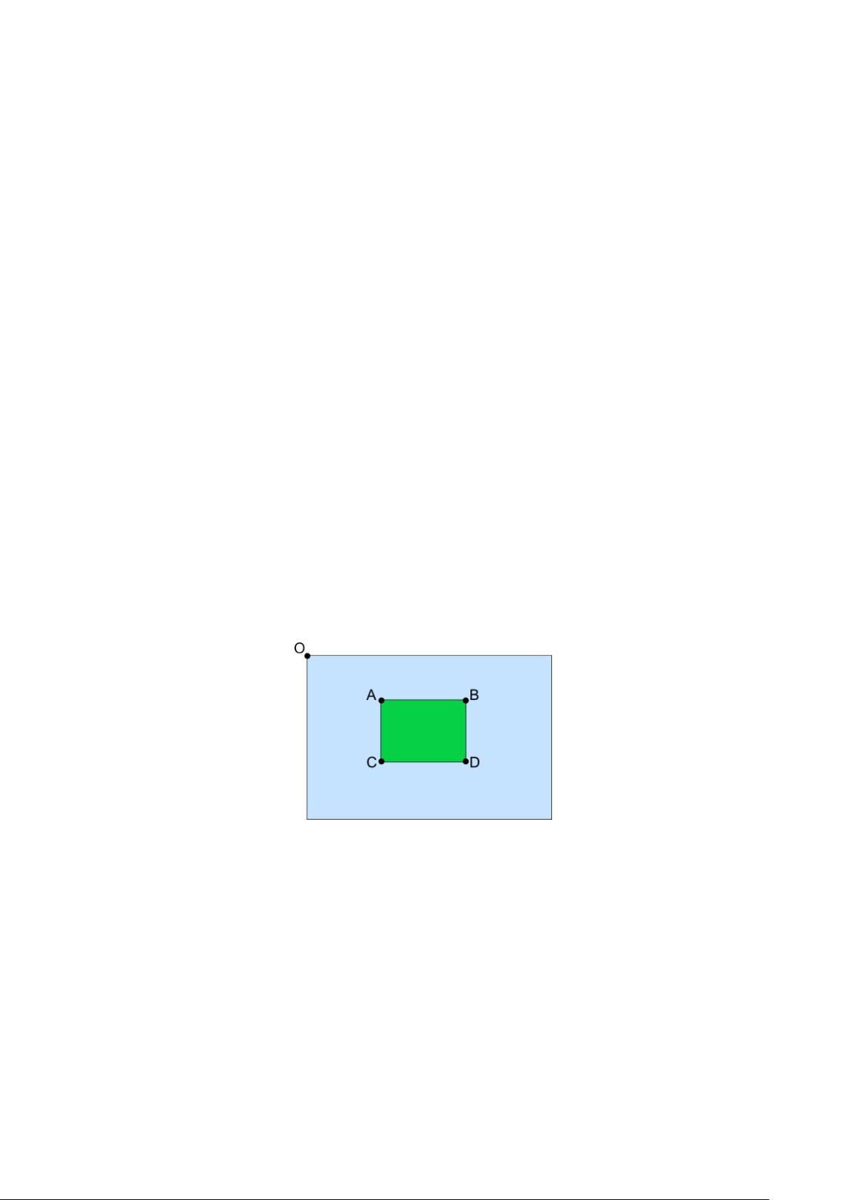
Figure 1: Area computation using integral images
Using the integral image, the task of calculating the area of an upright rectangular
region is reduced four operations. If we consider a rectangle bounded by vertices A, B,
C and D as in Figure 1, the sum of pixel intensities is calculated by:
X
= A + D − (C + B) (2)
Since computation time is invariant to change in size this approach is particularly useful
when large areas are required. SURF makes good use of this property to perform fast
convolutions of varying size box filters at near constant time.
1.2 Fast-Hessian Detector
1.2.1 The Hessian
The SURF detector is based on the determinant of the Hessian matrix. In order to
motivate the use of the Hessian, we consider a continuous function of two variables such
that the value of the function at (x, y) is given by f(x, y). The Hessian matrix, H, is the
matrix of partial derivates of the function f.
H(f(x, y)) =
"
∂
2
f
∂x
2
∂
2
f
∂x∂y
∂
2
f
∂x∂y
∂
2
f
∂y
2
#
(3)
The determinant of this matrix, known as the discriminant, is calculated by:
det(H) =
∂
2
f
∂x
2
∂
2
f
∂y
2
−
∂
2
f
∂x∂y
2
(4)
The value of the discriminant is used to classify the maxima and minima of the
function by the second order derivative test. Since the determinant is the product of
eigenvalues of the Hessian we can classify the points based on the sign of the result. If
the determinant is negative then the eigenvalues have different signs and hence the point
is not a local extremum; if it is positive then either both eigenvalues are positive or both
are negative and in either case the point is classified as an extremum.
Translating this theory to work with images rather than a continuous function is a
fairly trivial task. First we replace the function values f(x, y) by the image pixel intensi-
ties I(x, y). Next we require a method to calculate the second order partial derivatives of
the image. As described in Section ?? we can calculate derivatives by convolution with
an appropriate kernel. In the case of SURF the second order scale normalised Gaussian is
the chosen filter as it allows for analysis over scales as well as space (scale-space theory is
discussed further later in this section). We can construct kernels for the Gaussian deriva-
tives in x, y and combined xy direction such that we calculate the four entries of the
Hessian matrix. Use of the Gaussian allows us to vary the amount of smoothing during
the convolution stage so that the determinant is calculated at different scales. Further-
more, since the Gaussian is an isotropic (i.e. circularly symmetric) function, convolution
with the kernel allows for rotation invariance. We can now calculate the Hessian matrix,
H, as function of both space x = (x, y) and scale σ.
H(x, σ) =
"
L
xx
(x, σ) L
xy
(x, σ)
L
xy
(x, σ) L
yy
(x, σ)
#
, (5)
Here L
xx
(x, σ) refers to the convolution of the second order Gaussian derivative
∂
2
g(σ)
∂x
2
with the image at point x = (x, y) and similarly for L
yy
and L
xy
. These derivatives are
known as Laplacian of Gaussians.
Working from this we can calculate the determinant of the Hessian for each pixel in
the image and use the value to find interest points. This variation of the Hessian detector
is similar to that proposed by Beaudet [2].
Lowe [9] found performance increase in approximating the Laplacian of Gaussians by
a difference of Gaussians. In a similiar manner, Bay [1] proposed an approximation to
the Laplacian of Gaussians by using box filter representations of the respective kernels.
Figure 2 illustrates the similarity between the discretised and cropped kernels and their
box filter counterparts. Considerable performance increase is found when these filters
are used in conjunction with the integral image described in Section 1.1. To qauntify
the difference we can consider the number of array accesses and operations required in
the convolution. For a 9 × 9 filter we would require 81 array accesses and operations for
the original real valued filter and only 8 for the box filter representation. As the filter is
increased in size, the computation cost increases significantly for the original Laplacian
while the cost for the box filters is independent of size.
Figure 2: Laplacian of Gaussian Approximation. Top Row: The discretised and cropped second
order Gaussian derivatives in the x, y and xy-directions. We refer to these as L
xx
, L
yy
, L
xy
.
Bottom Row: Weighted Box filter approximations in the x, y and xy-directions. We refer to
these as D
xx
, D
yy
, D
xy
In Figure 2 the weights applied to each of the filter sections is kept simple. The
black regions are weighted with a value of 1, the white regions with a value of -1 and the
remaining areas not weighted at all. Simple weighting allows for rapid calculation of areas
but in using these weights we need to address the difference in response values between
the original and approximated kernels. Bay [1] proposes the following formula as an
accurate approximation for the Hessian determinant using the approximated Gaussians:
det(H
approx
) = D
xx
D
yy
− (0.9D
xy
)
2
(6)
In [1] the two filters are compared in detail and the results conclude that the box
representation’s negligible loss in accuracy is far outweighed by the considerable increase
in efficiency and speed. The determinant here is referred to as the blob response at
location x = (x, y, σ). The search for local maxima of this function over both space and
scale yields the interest points for an image. The exact method for extracting interest
points is explained in the following section.
1.2.2 Constructing the Scale-Space
In order to detect interest points using the determinant of Hessian it is first necessary to
introduce the notion of a scale-space. A scale-space is a continuous function which can be
used to find extrema across all possible scales [20]. In computer vision the scale-space is
typically implemented as an image pyramid where the input image is iteratively convolved
with Gaussian kernel and repeatedly sub-sampled (reduced in size). This method is used
to great effect in SIFT [9] but since each layer relies on the previous, and images need
to be resized it is not computationally efficient. As the processing time of the kernels
used in SURF is size invariant, the scale-space can be created by applying kernels of
increasing size to the original image. This allows for multiple layers of the scale-space
pyramid to be processed simultaneously and negates the need to subsample the image
hence providing performance increase. Figure 3 illustrates the difference between the
traditional scale-space structure and the SURF counterpart.
Figure 3: Filter Pyramid. The traditional approach to constructing a scale-space (left).
The image size is varied and the Guassian filter is repeatedly applied to smooth subse-
quent layers. The SURF approach (right) leaves the original image unchanged and varies
only the filter size.
The scale-space is divided into a number of octaves, where an octave refers to a series
of response maps of covering a doubling of scale. In SURF the lowest level of the scale-
space is obtained from the output of the 9 × 9 filters shown in 2. These filters correspond
to a real valued Gaussian with σ = 1.2. Subsequent layers are obtained by upscaling
the filters whilst maintaining the same filter layout ratio. As the filter size increases so
too does the value of the associated Gaussian scale, and since ratios of the layout remain
constant we can calculate this scale by the formula:
σ
approx
= Current Filter Size ·
Base Filter Scale
Base Filter Size
= Current Filter Size ·
1.2
9
When constructing larger filters, there are a number of factors which must be take into
consideration. The increase in size is restricted by the length of the positive and negative
lobes of the underlying second order Gaussian derivatives. In the approximated filters
the lobe size is set at one third the side length of the filter and refers to the shorter side
length of the weighted black and white regions. Since we require the presence of a central
pixel, the dimensions must be increased equally around this location and hence the lobe
size can increase by a minimum of 2. Since there are three lobes in each filter which must
be the same size, the smallest step size between consecutive filters is 6. For the D
xx
and
D
yy
filters the longer side length of the weighted regions increases by 2 on each side to
preserve structure. Figure 4 illustrates the structure of the filters as they increase in size.
Figure 4: Filter Structure. Subsequent filters sizes must differ by a minimum of 6 to
preserve filter structure.
剩余23页未读,继续阅读
资源评论
- shcnxjy2012-03-20应该是一份关于SURF算法的英文报告,很详细!
「已注销」
- 粉丝: 13
- 资源: 6
上传资源 快速赚钱
- 我的内容管理 展开
- 我的资源 快来上传第一个资源
- 我的收益 登录查看自己的收益
- 我的积分 登录查看自己的积分
- 我的C币 登录后查看C币余额
- 我的收藏
- 我的下载
- 下载帮助
最新资源
- 黑苹果OC引导-0.9.1
- Redis 服务等过期策略和内存淘汰策略解析
- debian配置FTP服务
- 基于Matlab和CPLEX的2变量机组组合调度程序(注释完全,可直接运行)(文档加Matlab源码)
- 基于TMS320F2812设计复合频率信号频率计AD09硬件(原理图+PCB )+CCS软件源码+详细设计文档资料.zip
- MultivariateAnalysis(目标规划、多元分析与插值的相关例子)(注释完全,可直接运行)(文档加Matlab源码)
- 黑苹果OC引导-0.9.2
- 数据库实验-王珊.doc
- unity读取excel工具 使用3.5即可
- Matplotlib 是一个 Python 的绘图库 Matplotlib 绘图指南与功能介绍.docx
资源上传下载、课程学习等过程中有任何疑问或建议,欢迎提出宝贵意见哦~我们会及时处理!
点击此处反馈
安全验证
文档复制为VIP权益,开通VIP直接复制
信息提交成功