


Objectives
4-1
4
4
Perceptron Learning Rule
Objectives 4-1
Theory and Examples 4-2
Learning Rules 4-2
Perceptron Architecture 4-3
Single-Neuron Perceptron 4-5
Multiple-Neuron Perceptron 4-8
Perceptron Learning Rule 4-8
Test Problem 4-9
Constructing Learning Rules 4-10
Unified Learning Rule 4-12
Training Multiple-Neuron Perceptrons 4-13
Proof of Convergence 4-15
Notation 4-15
Proof 4-16
Limitations 4-18
Summary of Results 4-20
Solved Problems 4-21
Epilogue 4-33
Further Reading 4-34
Exercises 4-36
Objectives
One of the questions we raised in Chapter 3 was: ÒHow do we determine the
weight matrix and bias for perceptron networks with many inputs, where
it is impossible to visualize the decision boundaries?Ó In this chapter we
will describe an algorithm for
training
perceptron networks, so that they
can
learn
to solve classification problems. We will begin by explaining what
a learning rule is and will then develop the perceptron learning rule. We
will conclude by discussing the advantages and limitations of the single-
layer perceptron network. This discussion will lead us into future chapters.
4
Perceptron Learning Rule
4-2
Theory and Examples
In 1943, Warren McCulloch and Walter Pitts introduced one of the first ar-
tificial neurons [McPi43]. The main feature of their neuron model is that a
weighted sum of input signals is compared to a threshold to determine the
neuron output. When the sum is greater than or equal to the threshold, the
output is 1. When the sum is less than the threshold, the output is 0. They
went on to show that networks of these neurons could, in principle, com-
pute any arithmetic or logical function. Unlike biological networks, the pa-
rameters of their networks had to be designed, as no training method was
available. However, the perceived connection between biology and digital
computers generated a great deal of interest.
In the late 1950s, Frank Rosenblatt and several other researchers devel-
oped a class of neural networks called perceptrons. The neurons in these
networks were similar to those of McCulloch and Pitts. RosenblattÕs key
contribution was the introduction of a learning rule for training perceptron
networks to solve pattern recognition problems [Rose58]. He proved that
his learning rule will always converge to the correct network weights, if
weights exist that solve the problem. Learning was simple and automatic.
Examples of proper behavior were presented to the network, which learned
from its mistakes. The perceptron could even learn when initialized with
random values for its weights and biases.
Unfortunately, the perceptron network is inherently limited. These limita-
tions were widely publicized in the book
Perceptrons
[MiPa69] by Marvin
Minsky and Seymour Papert. They demonstrated that the perceptron net-
works were incapable of implementing certain elementary functions. It
was not until the 1980s that these limitations were overcome with im-
proved (multilayer) perceptron networks and associated learning rules. We
will discuss these improvements in Chapters 11 and 12.
Today the perceptron is still viewed as an important network. It remains a
fast and reliable network for the class of problems that it can solve. In ad-
dition, an understanding of the operations of the perceptron provides a
good basis for understanding more complex networks. Thus, the perceptron
network, and its associated learning rule, are well worth discussion here.
In the remainder of this chapter we will define what we mean by a learning
rule, explain the perceptron network and learning rule, and discuss the
limitations of the perceptron network.
Learning Rules
As we begin our discussion of the perceptron learning rule, we want to dis-
cuss learning rules in general. By
learning rule
we mean a procedure for
modifying the weights and biases of a network. (This procedure may also
Learning Rule

Perceptron Architecture
4-3
4
be referred to as a training algorithm.) The purpose of the learning rule is
to train the network to perform some task. There are many types of neural
network learning rules. They fall into three broad categories: supervised
learning, unsupervised learning and reinforcement (or graded) learning.
In
supervised learning
, the learning rule is provided with a set of examples
(the
training set
) of proper network behavior:
, (4.1)
where is an input to the network and is the corresponding correct
(
target
) output. As the inputs are applied to the network, the network out-
puts are compared to the targets. The learning rule is then used to adjust
the weights and biases of the network in order to move the network outputs
closer to the targets. The perceptron learning rule falls in this supervised
learning category. We will also investigate supervised learning algorithms
in Chapters 7Ð12.
Reinforcement learning
is similar to supervised learning, except that, in-
stead of being provided with the correct output for each network input, the
algorithm is only given a grade. The grade (or score) is a measure of the net-
work performance over some sequence of inputs. This type of learning is
currently much less common than supervised learning. It appears to be
most suited to control system applications (see [BaSu83], [WhSo92]).
In
unsupervised learning
, the weights and biases are modified in response
to network inputs only. There are no target outputs available. At first
glance this might seem to be impractical. How can you train a network if
you donÕt know what it is supposed to do? Most of these algorithms perform
some kind of clustering operation. They learn to categorize the input pat-
terns into a finite number of classes. This is especially useful in such appli-
cations as vector quantization. We will see in Chapters 13Ð16 that there
are a number of unsupervised learning algorithms.
Perceptron Architecture
Before we present the perceptron learning rule, letÕs expand our investiga-
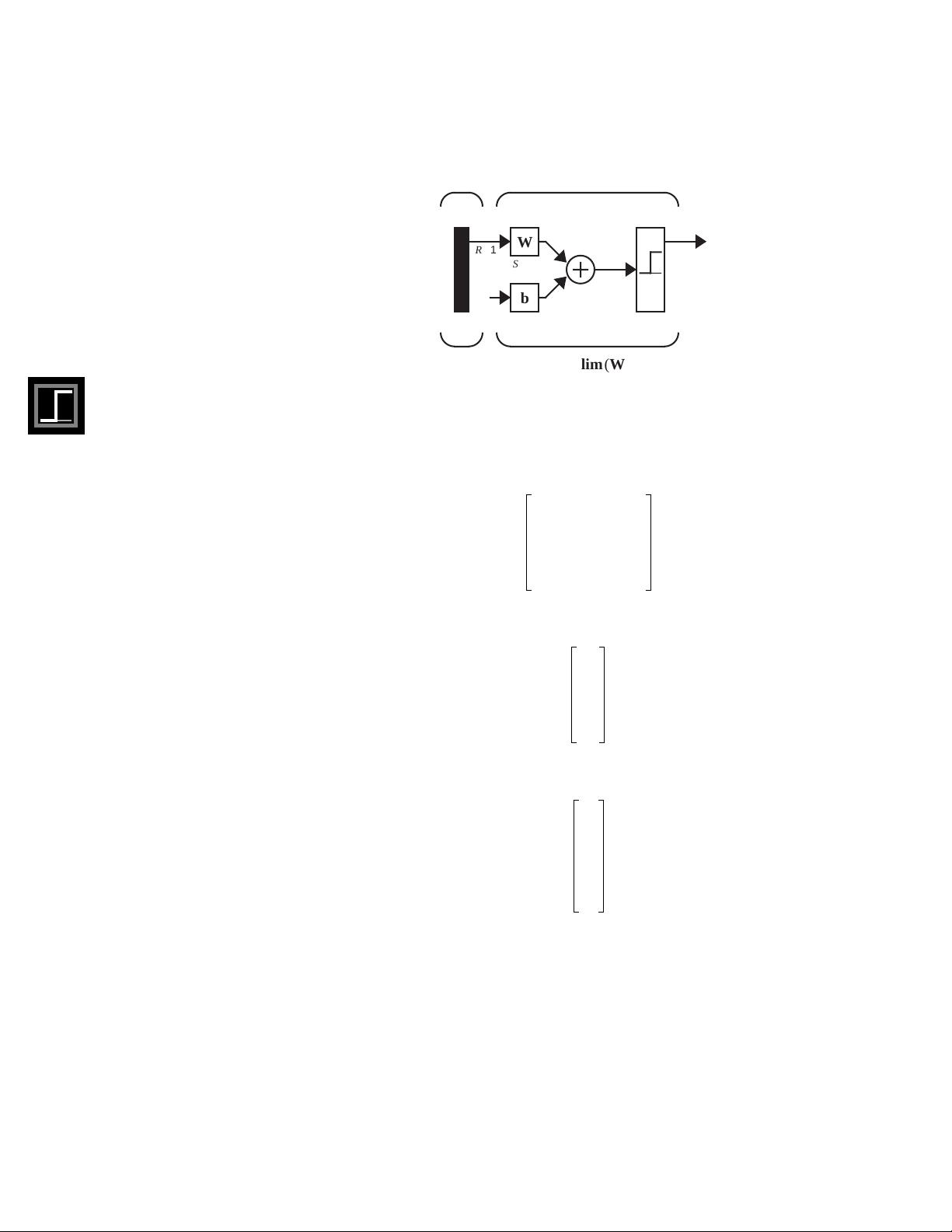
tion of the perceptron network, which we began in Chapter 3. The general
perceptron network is shown in Figure 4.1.
The output of the network is given by
. (4.2)
(Note that in Chapter 3 we used the transfer function, instead of
hardlim
. This does not affect the capabilities of the network. See Exercise
E4.6.)
Supervised Learning
Training Set
p
1
t
1
{,} p
2
t
2
{,}… p
Q
t
Q
{,},,,
p
q
t
q
Target
Reinforcement Learning
Unsupervised Learning
a hardlim Wp b+()=
hardlims
4
Perceptron Learning Rule
4-4
Figure 4.1 Perceptron Network
It will be useful in our development of the perceptron learning rule to be
able to conveniently reference individual elements of the network output.
LetÕs see how this can be done. First, consider the network weight matrix:
. (4.3)
We will define a vector composed of the elements of the
i
th row of :
. (4.4)
Now we can partition the weight matrix:
. (4.5)
This allows us to write the
i
th element of the network output vector as
pa
1
n
AA
AA
W
AA
AA
b
R x 1
S
x R
S
x 1
S
x 1
S
x 1
Input
RS
AA
AA
AA
a = hardlim (Wp + b)
Hard Limit Layer
W
w
11,
w
12,
… w
1 R,
w
21,
w
22,
… w
2 R,
w
S 1,
w
S 2,
… w
SR,
=
…
…
…
W
w
i
w
i 1,
w
i 2,
w
iR,
=
…
W
w
T
1
w
T
2
w
T
S
=
…
Perceptron Architecture
4-5
4
. (4.6)
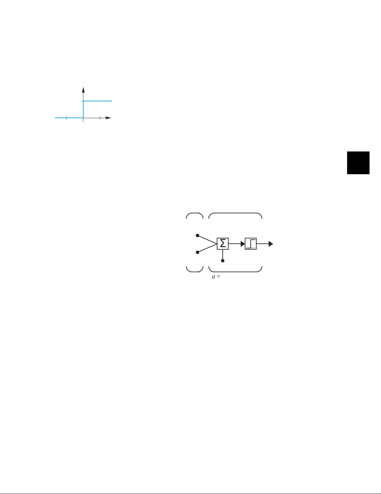
Recall that the transfer function (shown at left) is defined as:
(4.7)
Therefore, if the inner product of the
i
th row of the weight matrix with the
input vector is greater than or equal to , the output will be 1, otherwise
the output will be 0.
Thus each neuron in the network divides the input
space into two regions
. It is useful to investigate the boundaries between
these regions. We will begin with the simple case of a single-neuron percep-
tron with two inputs.
Single-Neuron Perceptron
LetÕs consider a two-input perceptron with one neuron, as shown in Figure
4.2.
Figure 4.2 Two-Input/Single-Output Perceptron
The output of this network is determined by
(4.8)
The
decision boundary
is determined by the input vectors for which the net
input is zero:
. (4.9)
To make the example more concrete, letÕs assign the following values for
the weights and bias:
a
i
hardlim n
i
() hardlim w
T
i
p b
i
+()==
hardlim
n = Wp + b
a = hardlim (n)
a hardlim n()
1 if n 0≥
0 otherwise.
==
b
i
–
p
1
an
Inputs
b
p
2
w
1,2
w
1,1
1
A
A
Σ
A
A
a = hardlim (Wp + b)
Two-Input Neuron
a hardlim n() hardlim Wp b+()==
hardlim w
T
1
p b+()hardlim w
11,
p
1
w
12,
p
2
b++()==
Decision Boundary
n
n w
T
1
p b+ w
11,
p
1
w
12,
p
2
b++0== =


