2013-Visualizing and Understanding Convolutional Networks
需积分: 16 142 浏览量
2015-05-21
10:14:00
上传
评论
收藏 34.56MB PDF 举报

Visualizing and Understanding Convolutional Networks
Matthew D. Zeiler zeiler@cs.nyu.edu
Dept. of Computer Science, Courant Institute, New York University
Rob Fergus fergus@cs.nyu.edu
Dept. of Computer Science, Courant Institute, New York University
Abstract
Large Convolutional Network models have
recently demonstrated impressive classifica-
tion performance on the ImageNet bench-
mark (Krizhevsky et al., 2012). However
there is no clear understanding of why they
perform so well, or how they might be im-
proved. In this paper we address both issues.
We introduce a novel visualization technique
that gives insight into the function of inter-
mediate feature layers and the operation of
the classifier. Used in a diagnostic role, these
visualizations allow us to find model architec-
tures that outperform Krizhevsky et al. on
the ImageNet classification benchmark. We
also perform an ablation study to discover
the performance contribution from different
model layers. We show our ImageNet model
generalizes well to other datasets: when the
softmax classifier is retrained, it convincingly
beats the current state-of-the-art results on
Caltech-101 and Caltech-256 datasets.
1. Introduction
Since their introduction by (LeCun et al., 1989) in
the early 1990’s, Convolutional Networks (convnets)
have demonstrated excellent performance at tasks such
as hand-written digit classification and face detec-
tion. In the last year, several papers have shown
that they can also deliver outstanding performance on
more challenging visual classification tasks. (Ciresan
et al., 2012) demonstrate state-of-the-art performance
on NORB and CIFAR-10 datasets. Most notably,
(Krizhevsky et al., 2012) show record beating perfor-
mance on the ImageNet 2012 classification benchmark,
with their convnet model achieving an error rate of
16.4%, compared to the 2nd place result of 26.1%.
Several factors are responsible for this renewed inter-
est in convnet models: (i) the availability of much
larger training sets, with millions of labeled exam-
ples; (ii) powerful GPU implementations, making the
training of very large models practical and (iii) bet-
ter model regularization strategies, such as Dropout
(Hinton et al., 2012).
Despite this encouraging progress, there is still lit-
tle insight into the internal operation and behavior
of these complex models, or how they achieve such
good performance. From a scientific standpoint, this
is deeply unsatisfactory. Without clear understanding
of how and why they work, the development of better
models is reduced to trial-and-error. In this paper we
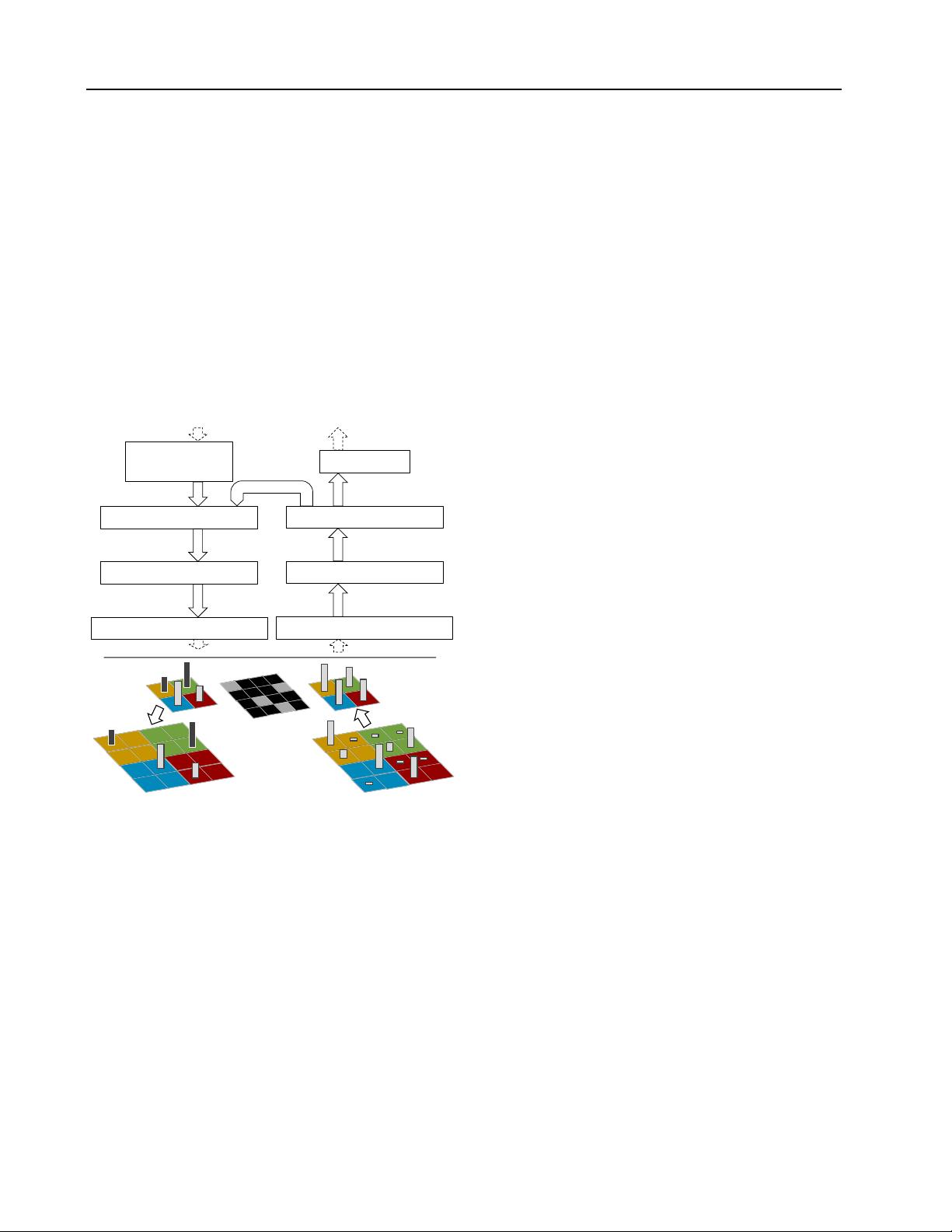
introduce a visualization technique that reveals the in-
put stimuli that excite individual feature maps at any
layer in the model. It also allows us to observe the
evolution of features during training and to diagnose
potential problems with the model. The visualization
technique we propose uses a multi-layered Deconvo-
lutional Network (deconvnet), as proposed by (Zeiler
et al., 2011), to project the feature activations back to
the input pixel space. We also perform a sensitivity
analysis of the classifier output by occluding portions
of the input image, revealing which parts of the scene
are important for classification.
Using these tools, we start with the architecture of
(Krizhevsky et al., 2012) and explore different archi-
tectures, discovering ones that outperform their results
on ImageNet. We then explore the generalization abil-
ity of the model to other datasets, just retraining the
softmax classifier on top. As such, this is a form of su-
pervised pre-training, which contrasts with the unsu-
pervised pre-training methods popularized by (Hinton
et al., 2006) and others (Bengio et al., 2007; Vincent
et al., 2008). The generalization ability of convnet fea-
tures is also explored in concurrent work by (Donahue
et al., 2013).
arXiv:1311.2901v3 [cs.CV] 28 Nov 2013

剩余10页未读,继续阅读
资源评论


lengwuqin
- 粉丝: 139
- 资源: 333


最新资源
- 最入门的爬虫代码 python.docx
- 爬虫零基础入门-爬取天气预报.pdf
- 最通俗易懂的 MongoDB 非结构化文档存储数据库教程.zip
- 以mongodb为数据库的订单物流小项目.zip
- 腾讯云-mongodb数据库, 项目部署.zip
- 腾讯 APIJSON 的 MongoDB 数据库插件.zip
- 理解非关系型数据库和关系型数据库的区别.zip
- 操作简单的Mongodb网页web管理工具,基于Spring Boot2.0支持mongodb集群.zip
- tms-mongodb-web,提供访问mongodb数据的REST API和可灵活扩展的mongodb web 客户端.zip
- SpringBoot整合mongodb学习MongoTemplate和MongoRepository两种方式CRUD使用.zip
资源上传下载、课程学习等过程中有任何疑问或建议,欢迎提出宝贵意见哦~我们会及时处理!
点击此处反馈


