


Full Terms & Conditions of access and use can be found at
http://www.tandfonline.com/action/journalInformation?journalCode=utch20
Download by: [South China University of Technology] Date: 07 May 2017, At: 19:55
Technometrics
ISSN: 0040-1706 (Print) 1537-2723 (Online) Journal homepage: http://www.tandfonline.com/loi/utch20
Multivariate SPC Charts for Monitoring Batch
Processes
Paul Nomikos & John F. MacGregor
To cite this article: Paul Nomikos & John F. MacGregor (1995) Multivariate SPC Charts for
Monitoring Batch Processes, Technometrics, 37:1, 41-59
To link to this article: http://dx.doi.org/10.1080/00401706.1995.10485888
Published online: 12 Mar 2012.
Submit your article to this journal
Article views: 173
View related articles
Citing articles: 25 View citing articles
@ 1995 American Statistical Association and
the American Society for Quality Control
TECHNOMETRICS, FEBRUARY 1995, VOL. 37, NO. 1
Multivariate SPC Charts for Monitoring Batch
Processes
Paul
NOMIKOS
and John F.
MACGREGOR
Department of Chemical Engineering
McMaster University
Hamilton, Ontario L8S 4L7
Canada
The problem of using time-varying trajectory data measured on many process variables over the finite
duration of a batch process is considered. Multiway principal-component analysis is used to compress
the information contained in the data trajectories into low-dimensional spaces that describe the operation
of past batches. This approach facilitates the analysis of operational and quality-control problems in
past batches and allows for the development of multivariate statistical process control charts for on-line
monitoring of the progress of new batches. Control limits for the proposed charts are developed using
information from the historical reference distribution of past successful batches. The method is applied
to data collected from an industrial batch polymerization reactor.
KEY WORDS: Control charts; On-line monitoring; Polymerization; Principal-component analysis;
Reference distribution; Statistical process control.
Batch and semi-batch processes play an important role
in the production and processing of high-quality speciality
materials and products. Examples include the production
of polymers, pharmaceuticals, and biochemicals; the sep-
aration and transformation of materials by batch distilla-
tion and crystallization; and the processing of materials
by injection molding. In general, a batch process is a
finite-duration process consisting of the following steps:
Charging of the batch vessel with a specified recipe of
materials; processing under controlled conditions during
which process variables such as temperatures, pressures,
agitation, and feedrates are varied according to specified
time trajectories; and finally discharging of the product.
On completion of the batch, a range of quality measure-
ments is usually made at the quality-control laboratory on
a sample of the product.
Batch processes generally exhibit some batch-to-batch
variation arising from such things as deviations of the pro-
cess variables from their specified trajectories, errors in the
charging of the recipe of materials, and disturbances aris-
ing from variations in impurities. Abnormal conditions
that develop during these batch operations can lead to the
production of at least one batch or a whole sequence of
batches with poor-quality product if the problem is not de-
tected and remedied. In spite of this, most industrial batch
processes are run without any effective form of real-time,
on-line monitoring to ensure that the batch is progress-
ing in a manner that will lead to a high-quality product
or to detect and indicate faults that can be corrected prior
to completion of the batch or can be corrected in sub-
sequent batches. For the most part, they rely simply on
the precise sequencing and automation of the major steps
in each batch run. Some effort has been made in indus-
try to use relational data base software to try to uncover
particular attributes of the measurement trajectories, such
as the timing of valve openings or the maximum tem-
perature or pressure attained during an interval, that ap-
pear to affect product quality and then to monitor these
attributes.
The application of statistical process control (SPC)
charts to batch processes has been very limited. Most
SPC methods use only the product quality measurements
obtained at the end of each batch (e.g., Vander Wiel,
Tucker, Faltin, and Doganaksoy 1992) and therefore mon-
itor only the batch-to-batch variation. Hahn and Cockrum
(1987) investigated the case in which one also has a few
quality measurements taken during the batch run. Marsh
and Tucker (1991) recognized that the process variable
measurements taken during a batch run, although tran-
sient in nature, do follow a certain dynamic pattern, and
they proposed a simple SPC technique for monitoring a
single measurement variable. Konstantinov and Yoshida
(1992) (temporal shapes of time profiles) and Holloway
and Krogh (1992) (trajectory encoding) applied qualita-
tive reasoning to tackle the monitoring problem of dy-
namic processes. Both tried to determine if the on-line
observations received from the process up to the present
time are consistent with some acceptable dynamic behav-
ior of the system. The lack of statistical reasoning in
their work and their univariate orientation are their main
drawbacks. Bonvin and Rippin (1990) used target-factor
analysis to identify on-line possible reaction stoichiome-
tries from measured composition or thermal data and to
detect any batch runaways (Prinz and Bonvin 1992).
41
42
PAUL NOMIKOS AND JOHN F. MACGREGOR
With on-line computers connected to most batch pro-
cesses, massive amounts of data are being collected rou-
tinely during the batch on many easily measured process
variables such as temperatures, pressures, and flowrates.
One may have measurements on up to 50 or more vari-
ables every few seconds throughout the entire history of a
batch. Furthermore, there is usually a history of many past
successful and some unsuccessful batches. Not only is the
relationship among all of the variables at any one time im-
portant, but so is the entire past history of the trajectories
of all these variables. The history of the process-variable
trajectories during a batch provide a “fingerprint” for each
batch, and it should be possible from these data to build an
empirical model to characterize the operation of success-
ful batch runs. The major difficulties are how to handle the
many measured process variables, their time-varying and
highly correlated structure, and the nonlinear finite-time
nature of batch operations.
To handle such large multivariable problems in continu-
ous processes operating around a fixed target, multivariate
SPC charts based on principal-component analysis (PCA)
and partial least squares or projection to latent struc-
tures (PLS) have been developed (Kresta, MacGregor, and
Marlin 1991; Skagerberg, MacGregor, and Kiparissides
1992; Miller, Swanson, and Heckler 1993; MacGre-
gor, Jaeckle, Kiparissides, and Koutoudi 1994). These
methods can use the many highly correlated process mea-
surements that are being continuously collected. The in-
formation contained in these data is projected into low-
dimensional spaces defined by latent vectors, and control
charts that are simple to present and easy to interpret have
been proposed and are now used in industry. Furthermore,
the diagnostic capabilities of these multivariate methods
have been shown to greatly enhance one’s ability to iso-
late assignable causes for violations of these charts (Miller
et al. 1993; MacGregor et al. 1994).
Recently MacGregor and Nomikos (1992) and
Nomikos and MacGregor (1994) employed multiway
PCA (MPCA) to extend multivariate SPC methods to
batch processes. By again projecting the information
contained in the process-variable trajectories down into
low-dimensional latent-variable spaces, both the variable
correlations and their time histories could be summa-
rized in a few plots. These multivariate approaches are
based on analyzing a historical reference distribution of
the measurement trajectories from past successful batches.
The variation in the trajectories among those batches
(common-cause variation) is characterized in a reduced
latent-vector space using MPCA. The behavior of new
batches is then compared to this reference distribution to
test the following hypothesis: H,: The on-line measure-
ments of the process-variable trajectories up to the current
time in a new batch are consistent with normal batch op-
eration as defined by the historical reference distribution.
The objectives of this article are (a) to present an
overview and some new variations of the MPCA method
TECHNOMETRICS, FEBRUARY 1995, VOL. 37, NO. 1
that have been proposed for the analysis and on-line moni-
toring of batch processes, (b) to establish statistical control
limits for the multivariate SPC charts that arise from these
methods, and (c) to illustrate the approach with an applica-
tion of the analysis and monitoring of an industrial batch
polymerization reactor.
The article is organized as follows. MPCA applied to
batch processes is outlined in Section 1, and its use in the
post-analysis of past batch polymerization runs is illus-
trated in Section 2. The selection of a suitable historical
reference distribution of past normal batches is illustrated
and modeled via MPCA in Section 3. Several varia-
tions of multivariate SPC charts for on-line monitoring
of the progress of new batches are presented in Section 4,
and statistical control limits for each of the multivariate
SPC charts are developed in Section 5. Two examples of
monitoring new batches are given in Section 6, and some
engineering issues and future directions are discussed in
Section 7.
1. MPCA FOR MODELING BATCH PROCESSES
Consider the problem at hand-namely, analyzing a his-
torical set of batch trajectory data. In a typical batch run,
j=l,2,..., J variables are measured at
k =
1,2, . . , K
time intervals throughout the batch. Similar data will ex-
ist on several (i = 1,2, . . , 1) similar process batch runs.
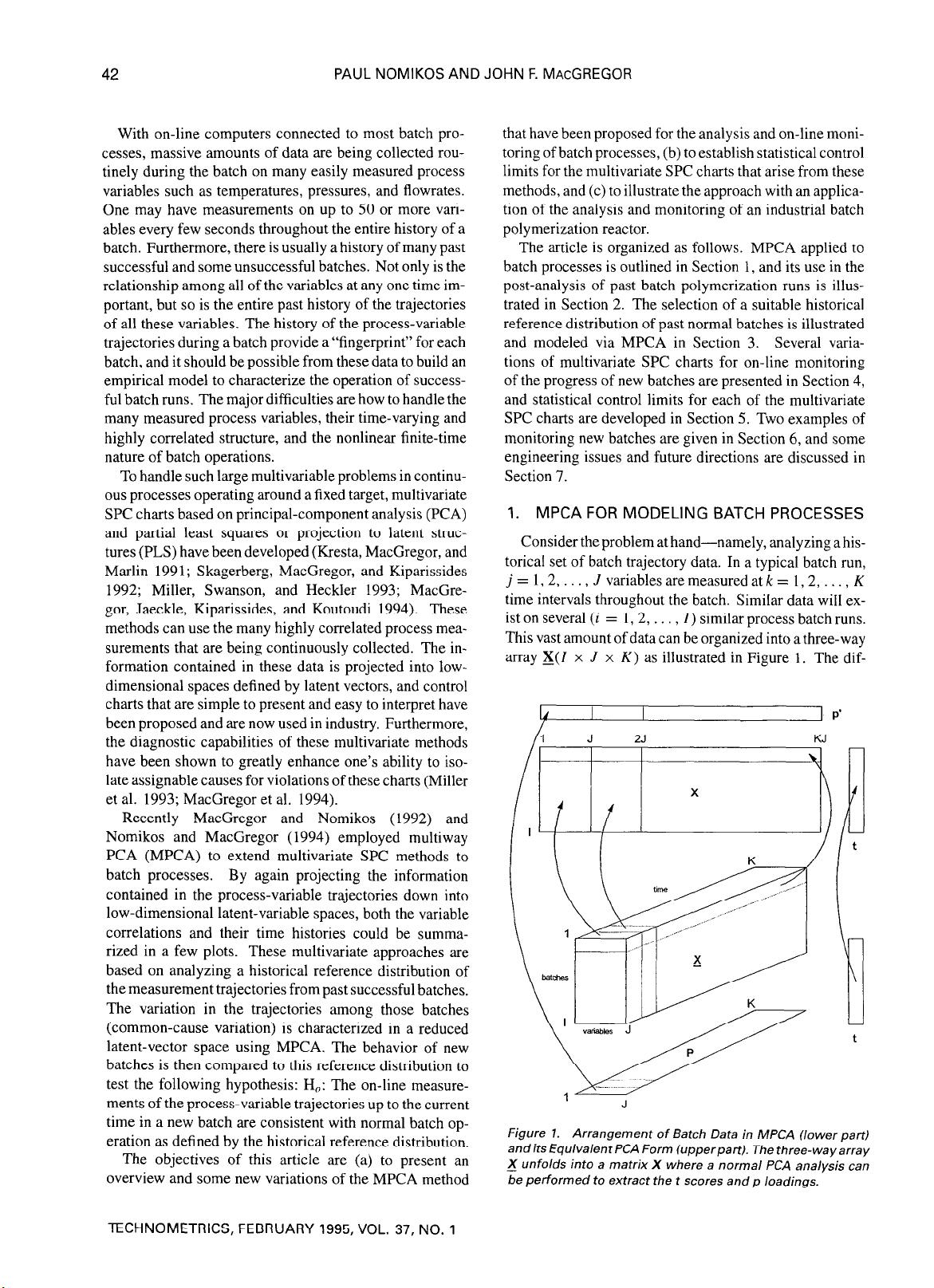
This vast amount of data can be organized into a three-way
array X(Z x J x
K)
as illustrated in Figure 1. The dif-
4 p’
Figure 1.
Arrangement of Batch Data in MPCA (lower part)
andits EquivalentPCA Form (upperpart). The three-wayarray
_X unfolds into a matrix X where a normal PCA analysis can
be performed to extract the t scores and p loadings.
MULTIVARIATE SPC CHARTS FOR MONITORING BATCH PROCESSES 43
ferent batch runs have been arranged along the vertical
axis, the measurement variables are across the horizontal
axis, and their time evolution occupies the third dimen-
sion. Each horizontal slice through this array is a (J x
K)
matrix containing the trajectories of all the variables from
a single batch (i). Each vertical slice is an (I x 1) ma-
trix representing the values of all the variables for all the
batches at a common time interval
(k).
Several multidimensional statistical methods have been
proposed for decomposing such data arrays into the sum
of a few products of vectors and matrices and to summa-
rize the variation of the data in the reduced dimensions of
these spaces. MPCA was introduced by Geladi, Esbenson,
and Ohman (1987) and was successfully applied in im-
age analysis (Geladi et al. 1989) and to some cases in
chemometrics (Smilde and Doornbos 1991). Other mul-
tiway methods (Geladi 1989) such as the Tucker model,
the PARAFAC model (Smilde and Doornbos 1991), the
canonical decomposition, the three-mode factor analysis
(Zeng and Hopke 1990), and the tensor rank (Sanchez
and Kowalski 1990) have been proposed for special sit-
uations. MacGregor and Nomikos (1992) and Nomikos
and MacGregor (1994), however, were able to show that
MPCA was well suited to handle multiway batch data.
MPCA is equivalent to unfolding the three-dimensional
array X slice by slice (three possible ways), rearranging
the slices into a large two-dimensional matrix X (two pos-
sible ways), and then performing a regular PCA. Each of
these six possible rearrangements of the data array X into
a large data matrix X, followed by a PCA on the matrix
X, corresponds to looking at a different type of variability.
For analyzing and monitoring batch processes, the most
meaningful way of unfolding the array X is to arrange
its vertical slices, corresponding to each point of time,
side by side into a two-dimensional matrix X(Z x
JK)
with the vertical slice corresponding to the first time in-
terval at the left side (Fig. 1). The data are then mean
centered and scaled prior to performing a PCA. This un-
folding is particularly meaningful because, by subtracting
the mean of each column of this matrix X, we are in effect
subtracting the mean trajectory of each variable, thereby
removing the main nonlinear and dynamic components in
the data. A PCA performed on these mean-corrected data
is therefore a study of the variation in the time trajectories
of all the variables in all batches about their mean tra-
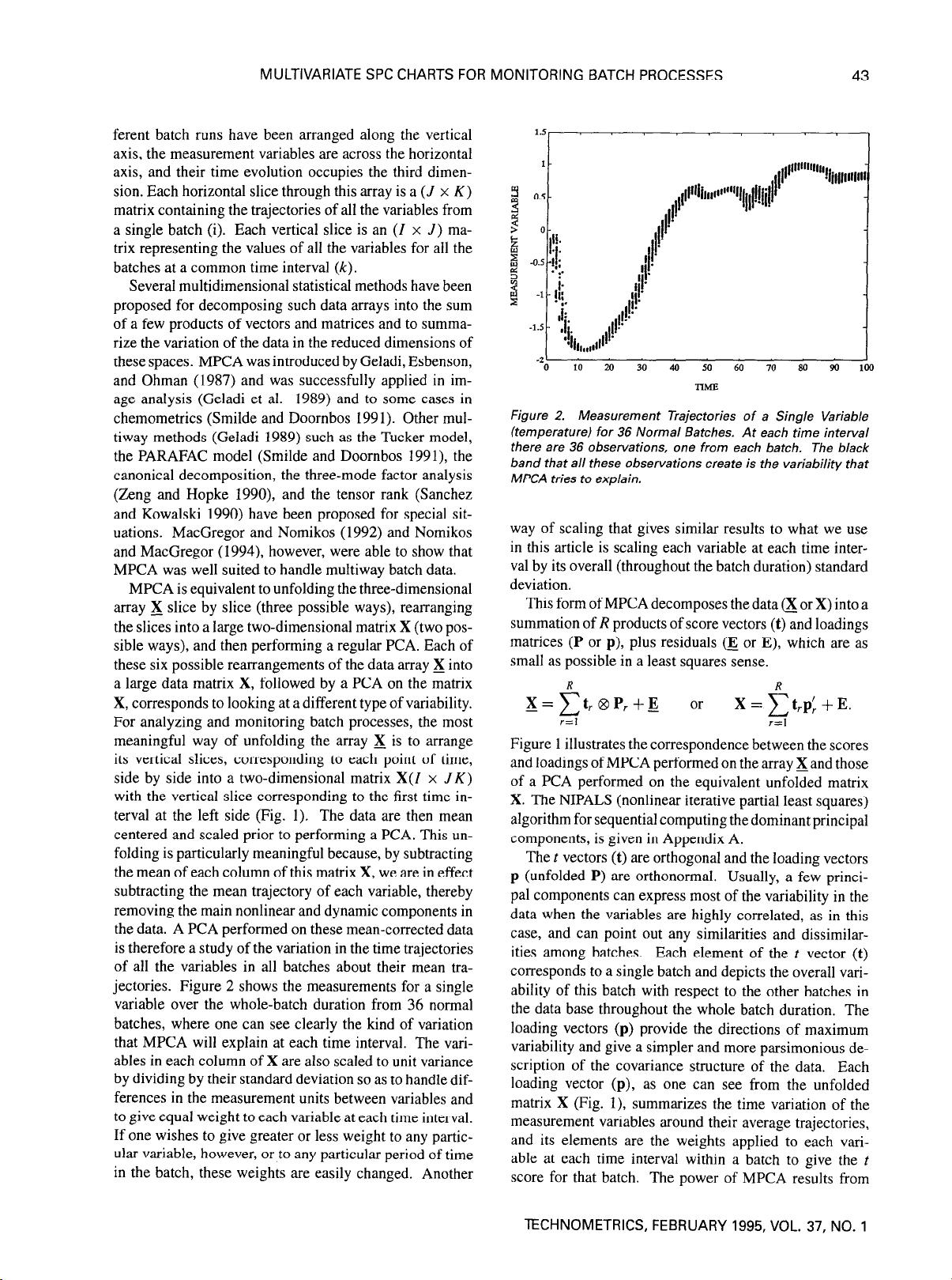
jectories. Figure 2 shows the measurements for a single
variable over the whole-batch duration from 36 normal
batches, where one can see clearly the kind of variation
that MPCA will explain at each time interval. The vari-
ables in each column of X are also scaled to unit variance
by dividing by their standard deviation so as to handle dif-
ferences in the measurement units between variables and
to give equal weight to each variable at each time interval.
If one wishes to give greater or less weight to any partic-
ular variable, however, or to any particular period of time
in the batch, these weights are easily changed. Another
J
0
10 20 30 40 50 60 70 80 90 loo
nhE
Figure 2. Measurement Trajectories of a Single Variable
(temperature) for 36 Normal Batches. At each time interval
there are 36 observations, one from each batch. The black
band that all these observations create is the variability that
MPCA tries to explain.
way of scaling that gives similar results to what we use
in this article is scaling each variable at each time inter-
val by its overall (throughout the batch duration) standard
deviation.
This form of MPCA decomposes the data a or X) into a
summation of
R
products of score vectors (t) and loadings
matrices (P or p), plus residuals (E or E), which are as
small as possible in a least squares sense.
X = f: t, 8 P, + E
or
X=f:t,p;+E.
i-=1
r=l
Figure 1 illustrates the correspondence between the scores
and loadings of MPCA performed on the array Xand those
of a PCA performed on the equivalent unfolded matrix
X. The NIPALS (nonlinear iterative partial least squares)
algorithm for sequential computing the dominant principal
components, is given in Appendix A.
The t vectors (t) are orthogonal and the loading vectors
p (unfolded P) are orthonormal. Usually, a few princi-
pal components can express most of the variability in the
data when the variables are highly correlated, as in this
case, and can point out any similarities and dissimilar-
ities among batches. Each element of the t vector (t)
corresponds to a single batch and depicts the overall vari-
ability of this batch with respect to the other batches in
the data base throughout the whole batch duration. The
loading vectors (p) provide the directions of maximum
variability and give a simpler and more parsimonious de-
scription of the covariance structure of the data. Each
loading vector (p), as one can see from the unfolded
matrix X (Fig. I), summarizes the time variation of the
measurement variables around their average trajectories,
and its elements are the weights applied to each vari-
able at each time interval within a batch to give the t
score for that batch. The power of MPCA results from
TECHNOMETRICS, FEBRUARY 1995, VOL. 37, NO. 1
44
PAUL NOMIKOS AND JOHN F. MACGREGOR
using the joint covariance matrix of the variable devia-
tions from their main trajectories. Thus it uses not just
the magnitude of the deviation of each variable from its
mean trajectory but also the contemporaneous correlation
among all of the variables over the time history of the
batches.
1 .l Selecting the Number of Principal
Components
The number of principal components needed to build
an MPCA model that describes adequately the normal
behavior of a batch operation can be found with several
criteria. These criteria range all the way from significance
tests to graphical procedures (Jackson 1991). One quick
and dirty criterion is the broken-stick rule (Jolliffe 1986).
This is based on the fact that if a line segment of unit length
is randomly divided into z segments the expected length
of the rth longest segment is
G = 100; $1/i.
I=r
As long as the percentage of variance explained by each
principal component is larger than the corresponding G,
then one can retain the corresponding principal compo-
nent. The number of segments is the maximum possible
rank of X, z = min(Z,
KJ),
and the rule should be ap-
plied only to unit variance-scaled matrices. This criterion
is rather crude but still is a quick method to judge if a prin-
cipal component adds any structural information about the
variance in the data or explains only noise.
When the purpose of a PCA analysis is to construct
a model that will be used on future observations, then
the suggested criterion to obtain the optimum number of
components is cross-validation (Efron 1983, 1986; Stone
1974). Cross-validation shows how the prediction power
of a PCA model increases as one adds more principal
components. It is a simple, but computationally lengthy,
procedure similar to the jackknifing method. Given a data
base of I normal batches with J variables and
K
time inter-
vals, the unfolded X matrix has dimensions Z x .Z
K.
After
scaling the matrix X, one batch is excluded from the data
base and a PCA model is built with the remaining (I - 1)
batches. This is done for all the batches in the data base,
and each time the sum of the squared prediction errors af-
ter each principal component is recorded for the batch not
included in the model building. At the end, these sum-of-
the-squared-prediction errors corresponding to each prin-
cipal component
(r)
are added for all the batches to give
the Press,.
One way to choose the model dimension is to select the
one with minimum Press, but this has been shown to have
poor statistical properties (Osten 1988). Wold (1978) and
Krzanowski (1983,1987) proposed two criteria for choos-
ing the optimal number of principal components. Wold
checked the ratio
R
= Press,/RSS,-i, where RSS, is
the residual sum of squares after the rth principal com-
TECHNOMETRICS, FEBRUARY 1995, VOL. 37, NO. 1
ponent based on the PCA model, which is built using the
whole data base. This criterion compares the prediction
power of a model based on
r
principal components with
the squared differences between observed and estimated
data using
r
- 1 principal components. A value of
R
larger
than unity suggests that the rth component did not improve
the prediction power of the model and it is better to use
only
r
- 1 components. Krzanowski suggested the ratio
W
= ((Press,-, - Press,)/&)/(Press,/Dr)
D,=Z+JK-2r
D, = JK(Z -
1) - 2Z +
JK - 2i,
i=l
where
D,
and
D,
are numbers indicating the degrees of
freedom required to fit the rth component and the degrees
of freedom remaining after fitting the rth component, re-
spectively. This statistic is similar to the F test for the
inclusion of an additional variable in a linear regression
model. It gives the ratio between the improvement in pre-
dictive power by adding the rth component and the pre-
dictive value of the same component. If
W
is larger than
unity, then this criterion suggests that the rth component
is worthwhile to be included in the model.
There is no sound statistical test for the cross-validation
procedure. The main problem is not knowing how many
degrees of freedom one starts with nor how many degrees
of freedom are extracted with each principal component
(e.g., Box, Hunter, MacGregor, and Erjavec 1973). Thus
the number of principal components needed in a PCA
model should be based on the overall picture that these
criteria give.
2. POST-ANALYSIS OF INDUSTRIAL
BATCH DATA
Data supplied by DuPont from an industrial batch poly-
merization reactor are used to illustrate the application of
the proposed method. The cycle in the reactor consists of
two stages, and the time spent processing in both stages is
approximately two hours. Ingredients are loaded into the
reactor to begin the first stage. Reactor-heating-medium
flows are adjusted to establish proper control of pressure
and the rate of temperature change. The solvent used to
convey ingredients to the reactor is vaporized and removed
from the reactor vessel. The vaporization process is vig-
orous enough that the contents of the vessel do not require
stirring. After nearly one hour spent removing solvent,
the second stage begins. During this stage the ingredi-
ents complete their reaction to yield the final product, a
polymer. Once again, vessel pressures and the rate of
temperature change are controlled during this processing
stage. The batch finishes by pumping the polymer product
from the vessel at the end of the second cycle.
The results of a critical property measurement are usu-
ally received 12 hours or more after each batch has fin-
ished, and therefore there is no time for recipe adjustments


