没有合适的资源?快使用搜索试试~ 我知道了~
LDPC编码的英文教材
5星 · 超过95%的资源 需积分: 11 33 下载量 154 浏览量
2010-05-02
20:58:24
上传
评论 1
收藏 1.76MB PDF 举报
温馨提示
试读
56页
有关LDPC编码的分类、构造以及解码,以具体的例子说明问题,深入浅出,适合初学者
资源推荐
资源详情
资源评论
5
Low-Density Parity-Check Codes
Low-density parity-check (LDPC) codes are a class of linear block codes with
implementable decoders which provide near-capacity performance on a large set
of data transmission and storage channels. LDPC codes were invented by Gal-
lager in his 1960 doctoral dissertation [1] and were mostly ignored in the 35 years
that followed. One notable exception is the important work of Tanner in 1981 [2]
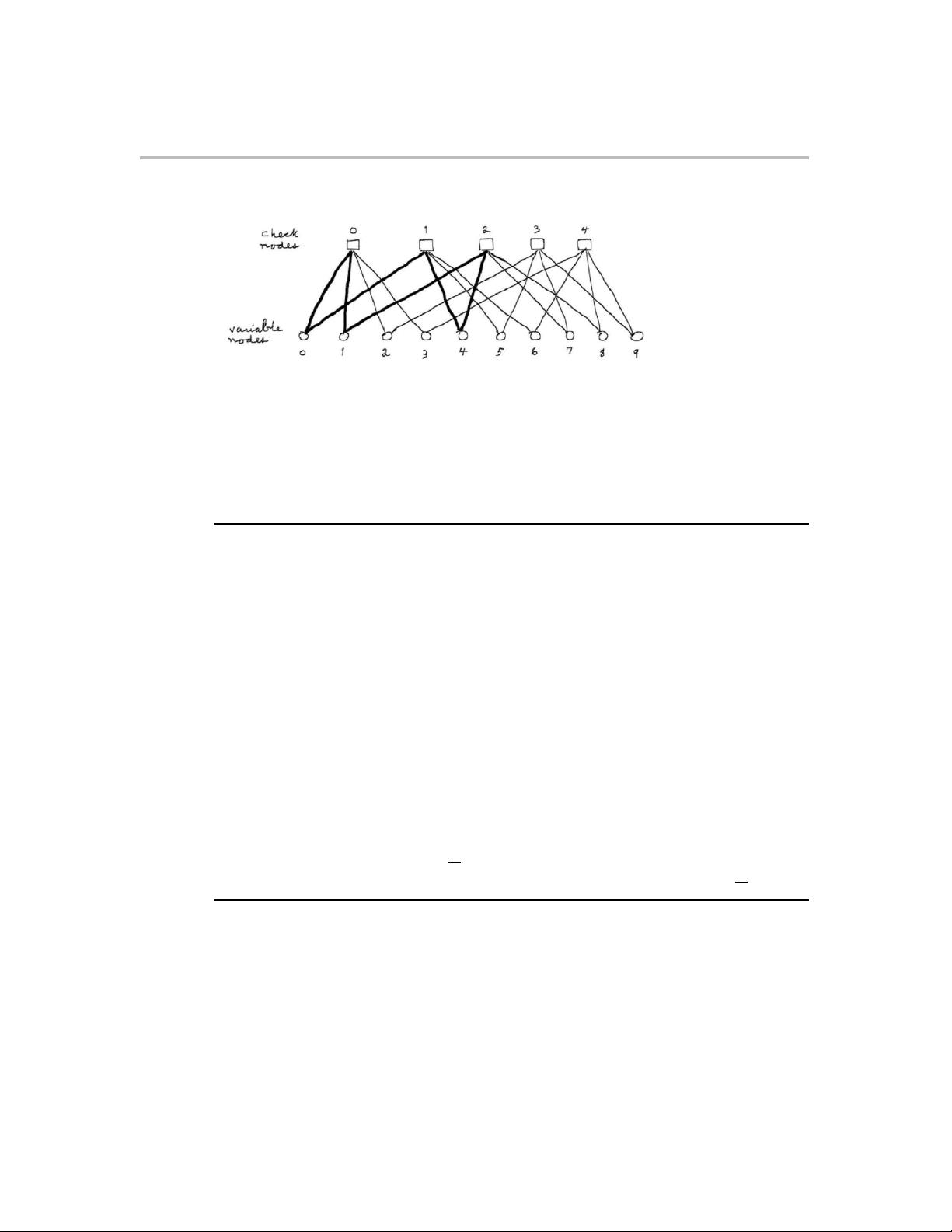
in which Tanner generalized LDPC codes and introduced a graphical representa-
tion of LDPC codes, now called a Tanner graph. The study of LDPC codes was
resurrected in the mid-1990’s with the work of MacKay, Luby, and others [3], [4],
[5], [6] who noticed, apparently independently of Gallager’s work, the advantages
of linear block codes with sparse (low-density) parity-check matrices.
This chapter introduces LDPC codes and creates a foundation for further study
of LDPC codes in later chapters. We start with the fundamental representations
of LDPC codes via parity-check matrices and Tanner graphs. We then learn
about the decoding advantages of linear codes which possess sparse parity-check
matrices. We will see that this sparse characteristic makes the code amenable
to various iterative decoding algorithms, which in many instances provide near-
optimal performance. Gallager [1] of course recognized the decoding advantages of
such low-density parity-check codes and he proposed a decoding algorithm for the
BI-AWGNC and a few others for the BSC. These algorithms have received much
scrutiny in the past decade, and are still being studied. In this chapter, we present
these decoding algorithms along with several others, most of which are related
to Gallager’s original algorithms. We point out that some of the algorithms were
independently obtained by other coding researchers (e.g., MacKay and Luby [4],
[5]), who were unaware of Gallager’s work at the time, as well as researchers
working on graph-based problems unrelated to coding [8].
5.1 Representations of LDPC Codes
5.1.1 Matrix Representation
We shall consider only binary LDPC codes for the sake of simplicity, although
LDPC codes can be generalized to non-binary alphabets as is done in Chapter
14. A low-density parity-check code is a linear block code given by the null space
1
2 Chapter 5. Low-Density Parity-Check Codes
of a m × n parity-check matrix H which has a low density of 1’s. A regular LDPC
code is a linear block code whose parity-check matrix H has column weight g and
row weight r, where r = g(n/m) and g << m. If H is low density, but its row and
column weight are not both constant, then the code is an irregular LDPC code.
For irregular LDPC codes, the various row and column weights are determined by
one of the code design procedures discussed in subsequent chapters. For reasons
that will become apparent later, almost all LDPC code constructions impose the
following additional structural property on H: no two rows (or two columns)
have more than one position in common which contains a nonzero element. This
property is called the row-column constraint, or simply, the RC-constraint.
The descriptor “low density” is unavoidably vague and cannot be precisely
quantified, although a density of 0.01 or lower can be called low density (1% or
lower of the entries of H are 1’s). As will be seen later in this chapter, the density
need only be sufficiently low to permit effective iterative decoding. This is in
fact the key innovation behind the invention of LDPC codes. As is well known,
optimum (e.g., maximum-likelihood) decoding of the general linear block code
that is useful for applications is not possible due to the vast complexity involved.
The low density aspect of LDPC codes accommodates iterative decoding which
typically has near-maximum-likelihood performance at error rates of interest for
many applications. These ideas will be made clearer as the student progresses
through this chapter.
As will be seen below and in later chapters, the construction of LDPC codes
usually involves the construction of H, which need not be full rank. In this case,
the code rate R for a regular LDPC code is bounded as
R ≥ 1 −
m
n
= 1 −
g
r
,
with equality when H is full rank.
5.1.2 Graphical Representation
The Tanner graph of an LDPC code is analogous to the trellis of a convolu-
tional code in that it provides a complete representation of the code and it aids
in the description of decoding algorithms. A Tanner graph is a bipartite graph
(introduced in Chapter 2), that is, a graph whose nodes may be separated into
two types, with edges connecting only nodes of different types. The two types of
nodes in a Tanner graph are the variable nodes (or code bit nodes) and the check
nodes (or constraint nodes), which we denote by VNs and CNs, respectively. The
Tanner graph of a code is drawn as follows: CN i is connected to VN j whenever
element h
ij
in H is a 1. Observe from this rule that there are m CNs in a Tanner
graph, one for each check equation, and n VNs, one for each code bit. Further,
the m rows of H specify the m CN connections, and the n columns of H specify
the n VN connections. Accordingly, the allowable n-bit words represented by the
n VNs are precisely the codewords in the code. Throughout this book, we shall
Low-Density Parity-Check Codes
3
Figure 5.1 Tanner graph for the code given in Example 5.1.
use both the notation CN i and VN j and the notation CN c
i
and VN v
j
, where
v
j
is the jth variable node or the jth code bit, depending on context.
Example 5.1: Consider a (10, 5) linear block code with w
c
= 2 and w
r
= 4 with the
following H matrix:
H =
1 1 1 1 0 0 0 0 0 0
1 0 0 0 1 1 1 0 0 0
0 1 0 0 1 0 0 1 1 0
0 0 1 0 0 1 0 1 0 1
0 0 0 1 0 0 1 0 1 1
.
The Tanner graph corresponding to H is depicted in Figure 5.1. Observe that VNs 0, 1,
2, and 3 are connected to CN 0 in accordance with the fact that, in the zeroth row of H,
h
00
= h
01
= h
02
= h
03
= 1 (all others are zero). Observe that analogous situations hold
for CNs 1, 2, 3, and 4 which correspond to rows 1, 2, 3, and 4 of H, respectively. Note,
as follows from vH
T
= 0, the bit values connected to the same check node must sum to
zero (mod 2). We may also proceed along columns to construct the Tanner graph. For
example, note that VN 0 is connected to CNs 0 and 1 in accordance with the fact that,
in the zeroth column of H, h
00
= h
10
= 1. The sum of rows of H is the all-zero vector,
so H is not full rank and R ≥ 1 −
5
10
. It is easily seen that the first row is dependent (it
is the sum of the other rows). From this, we have rank(H) = 4 and R = 1 −
4
10
= 3/5.
The Tanner graph of an LDPC code acts as a blueprint for the iterative decoder
in the following way. Each of the nodes acts as a locally operating processor and
each edge acts as a bus which conveys information from a given node to each
of its neighbors. The information conveyed is typically probabilistic information,
e.g., log-likelihood ratios (LLRs), pertaining to the values of the bits assigned to
the variable nodes. The LDPC decoder is initiated by n LLRs from the channel
which are received by the n VN processors. At the beginning of each half-iteration
in the basic iterative decoding algorithm, each VN processor takes inputs from
4 Chapter 5. Low-Density Parity-Check Codes
the channel and each of its neighboring CNs, and from these computes outputs
for each one of its neighboring CN processors. In the next half-iteration, each
CN processor takes inputs from each of its neighboring VNs, and from these
computes outputs for each one of its neighboring VN processors. The VN↔CN
iterations continue until a codeword is found or until the preset maximum number
of iterations has been reached.
The effectiveness of the iterative decoder depends on a number of structural
properties of the Tanner graph on which the decoder is based. Observe the six
thickened edges in Figure 5.1. A sequence of edges such as these which form
a closed path is called a cycle (see Chapter 2). We are interested in cycles
because short cycles degrade the performance of the iterative decoding algorithms
employed by LDPC codes. This fact will be made evident in the discussion of the
decoding algorithms later in this chapter, but it can also be seen from the brief
algorithm description in the previous paragraph. It should be clear from the
description that cycles force the decoder to operate locally in some portions of
the graph (e.g., continually around a short cycle) so that a globally optimum
solution is impossible. Observe also from the decoder description the necessity
of a low-density matrix H: at high densities (about half of the entries are 1’s),
many short cycles will exist, thus precluding the use of an iterative decoder.
The length of a cycle is equal to the number of edges which form the cycle
and so the length of the cycle in Figure 5.1 is six. A cycle of length l is often
called an l-cycle. The minimum cycle length in a given bipartite graph is called
the graph’s girth. The girth of the Tanner graph for the example co de is clearly
six. The shortest possible cycle in a bipartite graph is clearly a length-4 cycle,
and such cycles manifest themselves in the H matrix as four 1’s that lie on the
four corners of a rectangular submatrix of H. Observe that the RC-constraint
eliminates length-4 cycles.
The Tanner graph in the above example is regular: each VN has two edge
connections and each CN has four edge connections. We say that the degree of
each VN is 2 and the degree of each CN is 4. This is in accordance with the fact
that g = 2 and r = 4. It is also clear from this example that mr = ng must hold
for all regular LDPC codes since both mr and ng are equal to the number of
edges in the graph.
As will be shown in later chapters, it is possible to more closely approach
capacity limits with irregular LDPC codes than with regular LDPC codes. For
irregular LDPC codes, the parameters g and r vary with the columns and rows,
so such notation is not useful in this case. Instead, it is usual in the literature
to specify the VN and CN degree distribution polynomials, denoted by λ(X) and
ρ(X), respectively. In the polynomial
λ(X) =
d
v
X
d=1
λ
d
X
d−1
, (5.1)
Low-Density Parity-Check Codes
5
λ
d
denotes the fraction of all edges connected to degree-d VNs and d
v
denotes
the maximum VN degree. Similarly, in the polynomial
ρ(X) =
d
c
X
d=1
ρ
d
X
d−1
, (5.2)
ρ
d
denotes the fraction of all edges connected to degree-d CNs and d
c
denotes
the maximum CN degree. Note, for the regular code above, for which g = 2 and
r = 4, we have λ(X) = X and ρ(X) = X
3
.
Let us denote the number of VNs of degree d by N
v
(d) and the number of CNs
of degree d by N
c
(d). Let us further denote by E the number of edges in the
graph. Then it can be shown that
E =
n
R
1
0
λ(X)dX
=
m
R
1
0
ρ(X)dX
(5.3)
N
v
(d) = Eλ
d
/d =
nλ
d
/d
R
1
0
λ(X)dX
(5.4)
N
c
(d) = Eρ
d
/d =
mρ
d
/d
R
1
0
ρ(X)dX
. (5.5)
From the two expressions for E we may easily conclude that the code rate is
bounded as
R ≥ 1 −
m
n
= 1 −
R
1
0
ρ(X)dX
R
1
0
λ(X)dX
. (5.6)
The polynomials λ(X) and ρ(X) represent a Tanner graph’s degree distribu-
tions from an “edge perspective”. The degree distributions may also be repre-
sented from a “node perspective” using the notation
˜
λ(X) and ˜ρ(X), where the
coefficient
˜
λ
d
is the fraction of all VNs that have degree d and ˜ρ
d
is the fraction
of CNs that have degree d. It is easily shown that
˜
λ
d
=
λ
d
/d
R
1
0
λ(X)dX
, (5.7)
˜ρ
d
=
ρ
d
/d
R
1
0
ρ(X)dX
. (5.8)
5.2 Classifications of LDPC Codes
As described in the next chapter, the original LDPC codes are random in the
sense that their parity-check matrices possess little structure. This is problem-
atic in that both encoding and decoding becomes quite complex when the code
possesses no structure beyond being a linear code. More recently, LDPC codes
with structure have been constructed.
剩余55页未读,继续阅读
资源评论
- guoyifeng552014-07-23正好在写LDPC的论文,用的着
chen07274032
- 粉丝: 1
- 资源: 13
上传资源 快速赚钱
- 我的内容管理 展开
- 我的资源 快来上传第一个资源
- 我的收益 登录查看自己的收益
- 我的积分 登录查看自己的积分
- 我的C币 登录后查看C币余额
- 我的收藏
- 我的下载
- 下载帮助
安全验证
文档复制为VIP权益,开通VIP直接复制
信息提交成功