没有合适的资源?快使用搜索试试~ 我知道了~
LabView2011控制设计与仿真基础篇
4星 · 超过85%的资源 需积分: 9 33 下载量 197 浏览量
2011-11-15
12:35:55
上传
评论 1
收藏 2.37MB PDF 举报
温馨提示
试读
77页
LabView2011控制设计与仿真基础篇详细的讲解了在labView中控制与仿真的技术
资源推荐
资源详情
资源评论
控 制 设 计 与 仿 真 概 念 篇
LabVIEW
开发技术丛书
目 录
目 录
Modeling a System 1-6
PID Control 7-16
Root Locus for Control Systems 17-22
Frequency Response for Control Systems 23-39
State-Space Design Method for Control Systems 40-56
Digital Control 57-66
Simulation Modeling for Control Systems 67-75
1
Modeling a System
Train System
In this example, we will consider a toy train consisting of an engine and a car. Assuming that the train only travels in
one direction, we want to apply control to the train so that it has a smooth start-up and stop, along with a constant-
speed ride.
The mass of the engine and the car will be represented by M1 and M2, respectively. The two are held together by a
spring, which has the stiffness coefficient of k. F represents the force applied by the engine, and the Greek letter, mu
(which will also be represented by the letter u), represents the coefficient of rolling friction.
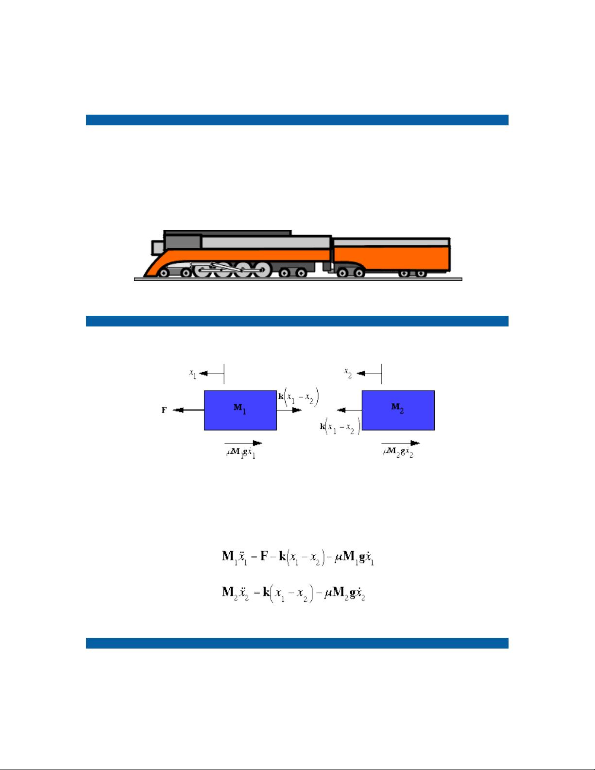
Free Body Diagram and Newton's Law
The system can be represented by following Free Body Diagrams.
Figure 1: Free Body Diagrams
From Newton's law, you know that the sum of forces acting on a mass equals the mass times its acceleration. In this
case, the forces acting on M1 are the spring, the friction and the force applied by the engine. The forces acting on M2
are the spring and the friction. In the vertical direction, the gravitational force is canceled by the normal force applied
by the ground, so that there will be no acceleration in the vertical direction. The equations of motion in the horizontal
direction are the following:
State-variable and Output Equations
This set of system equations can now be manipulated into state-variable form. The state variables are the positions,
X1 and X2, and the velocities, V1 and V2; the input is F. The state variable equations will look like the following:
2
Let the output of the system be the velocity of the engine. Then the output equation will be:
Transfer Function
To find the transfer function of the system, we first take the Laplace transforms of the differential equations.
The output is Y(s) = V1(s) = s X1(s). The variable X1 should be algebraically eliminated to leave an expression for
Y(s)/F(s). When finding the transfer function, zero initial conditions must be assumed. The transfer function should
look like the one shown below.
LabVIEW Graphical Approach
If you choose to use the transfer function, create a blank VI and add the CD Construct Transfer Function Model VI to
your block diagram. This VI is located in the Model Construction section of the Control Design palette.
Click the drop-down box that shows “SISO” and select “Single-Input Single-Output (Symbolic)”. To create inputs for
this transfer function, right-click on the Symbolic Numerator terminal and select Create » Control. Repeat this for the
Symbolic Denominator and Variables terminals. These controls will now appear on the front panel.
Figure 2: Create Transfer Function
Next, add the CD Draw Transfer Function VI to your block diagram, located in the Model Construction section of the
Control Design palette. Connect the Transfer Function Model output from the CD Create Transfer Function Model VI
to the Transfer Function Model input on the CD Draw Transfer Function VI.
3
Finally, create an indicator from the CD Draw Transfer Function VI. To do this, right-click on the Equation terminal and
select Create»Indicator.
Figure 3: Display Transfer Function
Now create a While Loop, located in the Structures palette, and surround all of the code in the block diagram. Next,
right-click on the Loop Condition terminal in the bottom-right corner of the While Loop, and select Create»Control.
Figure 4: Transfer Function with While Loop
With this VI, you can now create a transfer function for the train system. Try changing the numerator and the
denominator in the front panel, and observe the effects on the transfer function equation.
Figure 5: Transfer Function Front Panel (Download)
State-Space Model
Another method to solve the problem is to use the state-space form. Four matrices A, B, C, and D characterize the
system behavior and will be used to solve the problem. The state-space form which is found from the state-variable
and the output equations is shown below.
剩余76页未读,继续阅读
资源评论
- yangshijieabab2013-12-08英文版的啊。。。也可以,谢谢啦。。。
- soundb2012-07-26English only.
amoxiaoer
- 粉丝: 0
- 资源: 3
上传资源 快速赚钱
- 我的内容管理 展开
- 我的资源 快来上传第一个资源
- 我的收益 登录查看自己的收益
- 我的积分 登录查看自己的积分
- 我的C币 登录后查看C币余额
- 我的收藏
- 我的下载
- 下载帮助
安全验证
文档复制为VIP权益,开通VIP直接复制
信息提交成功