


H.1
Introduction H-2
H.2
Basic Techniques of Integer Arithmetic H-2
H.3
Floating Point H-13
H.4
Floating-Point Multiplication H-17
H.5
Floating-Point Addition H-21
H.6
Division and Remainder H-27
H.7
More on Floating-Point Arithmetic H-33
H.8
Speeding Up Integer Addition H-37
H.9
Speeding Up Integer Multiplication and Division H-45
H.10
Putting It All Together H-58
H.11
Fallacies and Pitfalls H-62
H.12
Historical Perspective and References H-63
Exercises H-69
H
Computer Arithmetic
by David Goldberg
Xerox Palo Alto Research Center
The Fast drives out the Slow even if the Fast is wrong.
W. Kahan
© 2003 Elsevier Science (USA). All rights reserved.

H-2
■
Appendix H
Computer Arithmetic
Although computer arithmetic is sometimes viewed as a specialized part of CPU
design, it is a very important part. This was brought home for Intel in 1994 when
their Pentium chip was discovered to have a bug in the divide algorithm. This
floating-point flaw resulted in a flurry of bad publicity for Intel and also cost them
a lot of money. Intel took a $300 million write-off to cover the cost of replacing
the buggy chips.
In this appendix we will study some basic floating-point algorithms, includ-
ing the division algorithm used on the Pentium. Although a tremendous variety of
algorithms have been proposed for use in floating-point accelerators, actual
implementations are usually based on refinements and variations of the few basic
algorithms presented here. In addition to choosing algorithms for addition, sub-
traction, multiplication, and division, the computer architect must make other
choices. What precisions should be implemented? How should exceptions be
handled? This appendix will give you the background for making these and other
decisions.
Our discussion of floating point will focus almost exclusively on the IEEE
floating-point standard (IEEE 754) because of its rapidly increasing acceptance.
Although floating-point arithmetic involves manipulating exponents and shifting
fractions, the bulk of the time in floating-point operations is spent operating on
fractions using integer algorithms (but not necessarily sharing the hardware that
implements integer instructions). Thus, after our discussion of floating point, we
will take a more detailed look at integer algorithms.
Some good references on computer arithmetic, in order from least to most
detailed, are Chapter 4 of Patterson and Hennessy [1994]; Chapter 7 of Hama-
cher, Vranesic, and Zaky [1984]; Gosling [1980]; and Scott [1985].
Readers who have studied computer arithmetic before will find most of this sec-
tion to be review.
Ripple-Carry Addition
Adders are usually implemented by combining multiple copies of simple com-
ponents. The natural components for addition are
half adders
and
full adders
.
The half adder takes two bits
a
and
b
as input and produces a sum bit
s
and a
carry bit
c
out
as output. Mathematically,
s
= (
a
+
b
) mod 2
,
and
c
out
=
(
a
+
b
)/2
,
where
is the floor function. As logic equations,
s
=
ab
+
ab
and
c
out
=
ab
,
where
ab
means
a
∧
b
and
a
+
b
means
a
∨
b
. The half adder is also called a (2,2)
adder, since it takes two inputs and produces two outputs. The full adder is a
(3,2) adder and is defined by
s
= (
a
+
b
+
c
) mod 2,
c
out
=
(
a
+
b
+
c
)/2
, or the
logic equations
H.1 Introduction
H.2 Basic Techniques of Integer Arithmetic

H.2 Basic Techniques of Integer Arithmetic
■
H
-
3
H.2.1
s
=
ab
c
+
a
bc
+
a
bc
+
abc
H.2.2
c
out
=
ab
+
ac
+
bc
The principal problem in constructing an adder for
n
-bit numbers out of
smaller pieces is propagating the carries from one piece to the next. The most
obvious way to solve this is with a
ripple-carry adder,
consisting of
n
full
adders, as illustrated in Figure H.1. (In the figures in this appendix, the least-sig-
nificant bit is always on the right.) The inputs to the adder are
a
n
–1
a
n
–2
⋅ ⋅ ⋅
a
0
and
b
n
–1
b
n
–2
⋅ ⋅ ⋅
b
0
, where
a
n
–1
a
n
–2
⋅ ⋅ ⋅
a
0
represents the number
a
n
–1
2
n
–1
+
a
n
–2
2
n
–2
+
⋅ ⋅ ⋅
+
a
0
. The
c
i
+1
output of the
i
th adder is fed into the
c
i
+1
input of the
next adder (the (
i
+ 1)-th adder) with the lower-order carry-in
c
0
set to 0. Since
the low-order carry-in is wired to 0, the low-order adder could be a half adder.
Later, however, we will see that setting the low-order carry-in bit to 1 is useful
for performing subtraction.
In general, the time a circuit takes to produce an output is proportional to the
maximum number of logic levels through which a signal travels. However, deter-
mining the exact relationship between logic levels and timings is highly technol-
ogy dependent. Therefore, when comparing adders we will simply compare the
number of logic levels in each one. How many levels are there for a ripple-carry
adder? It takes two levels to compute
c
1
from
a
0
and
b
0
. Then it takes two more
levels to compute
c
2
from
c
1
,
a
1
,
b
1
, and so on, up to
c
n
. So there are a total of 2
n
levels. Typical values of
n
are 32 for integer arithmetic and 53 for double-
precision floating point. The ripple-carry adder is the slowest adder, but also the
cheapest. It can be built with only
n
simple cells, connected in a simple, regular
way.
Because the ripple-carry adder is relatively slow compared with the designs
discussed in Section H.8, you might wonder why it is used at all. In technologies
like CMOS, even though ripple adders take time O(
n
), the constant factor is very
small. In such cases short ripple adders are often used as building blocks in larger
adders.
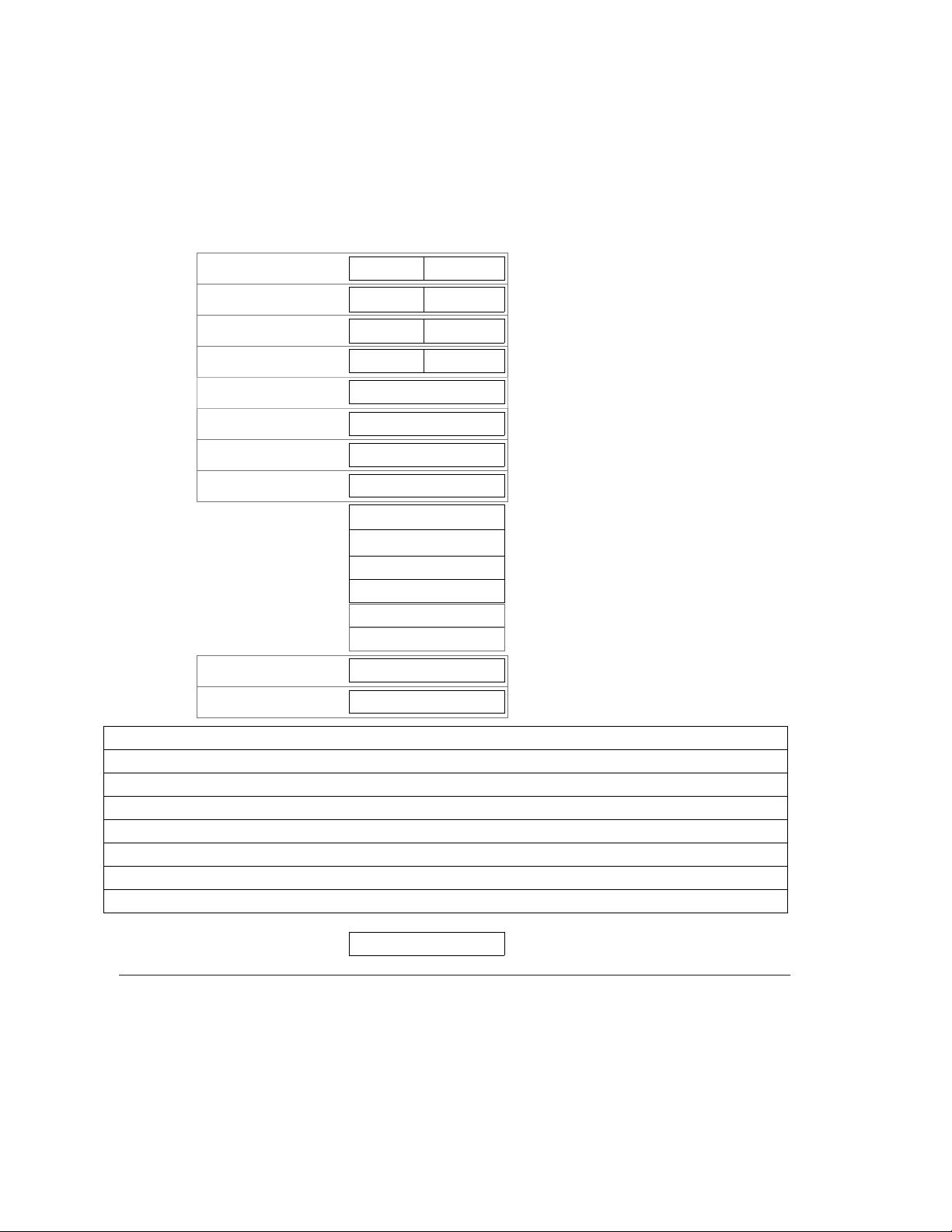
Figure H.1 Ripple-carry adder, consisting of n full adders.The carry-out of one full
adder is connected to the carry-in of the adder for the next most-significant bit. The car-
ries ripple from the least-significant bit (on the right) to the most-significant bit (on the
left).
b
n–1
a
n–1
s
n–1
Full
adder
c
n–1
s
n–2
c
n
a
n–2
b
n–2
Full
adder
b
1
a
1
s
1
Full
adder
s
0
a
0
b
0
Full
adder
c
2
c
1
0
H-4 ■ Appendix H Computer Arithmetic
Radix-2 Multiplication and Division
The simplest multiplier computes the product of two unsigned numbers, one bit at
a time, as illustrated in Figure H.2(a). The numbers to be multiplied are a
n–1
a
n–2
⋅ ⋅ ⋅ a
0
and b
n–1
b
n–2
⋅ ⋅ ⋅ b
0
, and they are placed in registers A and B, respectively.
Register P is initially 0. Each multiply step has two parts.
Multiply Step (i) If the least-significant bit of A is 1, then register B, containing b
n–1
b
n–2
⋅ ⋅ ⋅
b
0
, is added to P; otherwise 00 ⋅ ⋅ ⋅ 00 is added to P. The sum is placed back
into P.
Figure H.2 Block diagram of (a) multiplier and (b) divider for n-bit unsigned inte-
gers. Each multiplication step consists of adding the contents of P to either B or 0
(depending on the low-order bit of A), replacing P with the sum, and then shifting both
P and A one bit right. Each division step involves first shifting P and A one bit left, sub-
tracting B from P, and, if the difference is nonnegative, putting it into P. If the difference
is nonnegative, the low-order bit of A is set to 1.
Carry-out
PA
n
n
n
Shift
P
B0
A
n + 1
n1
n
Shift
(a)
(b)
1
B


