


Project 2: Message Passing
A report submitted in fulfillment of
requirement for project 2 of
Networks & Parallel Processing (433677)
2 Semester 2009
By
Group 15
Minghai Gao (ID: 352844)
Li Zhun Wang (ID: 354860)
2
Abstract:
Heat distribution problem in 2 dimensions can be
described by Laplace’s equation and the finite
element method generates an approximate solution
can be implemented by iterative solutions called
Jacobi’s iterations. In order to learn and study the
heat distribution in 2 dimensions problems’
implementations of iterative solutions by using both
sequential algorithm and parallel algorithm. We made
two kinds of algorithms, one is sequential
implementation of this iterative solution, the other is
parallel implementation. And we compared and
contrasted these implementations in terms of latency,
efficiency and complexity in this report.
1. Introduction:
Using Laplace’s equation:
We can describe the heat distribution in 2 dimensions
problem.
We defined a Matrix, H, where h
i,j
(the i-th row and
j-th column of A) is the temperature at that element.
h
1,1
h
1,2
h
1,3
… h
1,n
h
2,1
h
2,2
h
2,3
… h
2,n
H = h
3,1
h
3,2
h
3,3
… h
3,n
… … … … … …
h
n,1
h
n,2
h
n,3
… h
n,n
The finite element method generates an approximate
solution by iteratively averaging the temperature of
elements until the maximum change of an element is
less than some ε>0:
[4]
(1)
And we can use the following equation to get the
value of the maximum change, we call it as variance.
When variance is less than ε² the distribution of heat
will stop computing as follows:
Additional the appropriate boundary conditions must
be known and remain constant throughout the
computations.
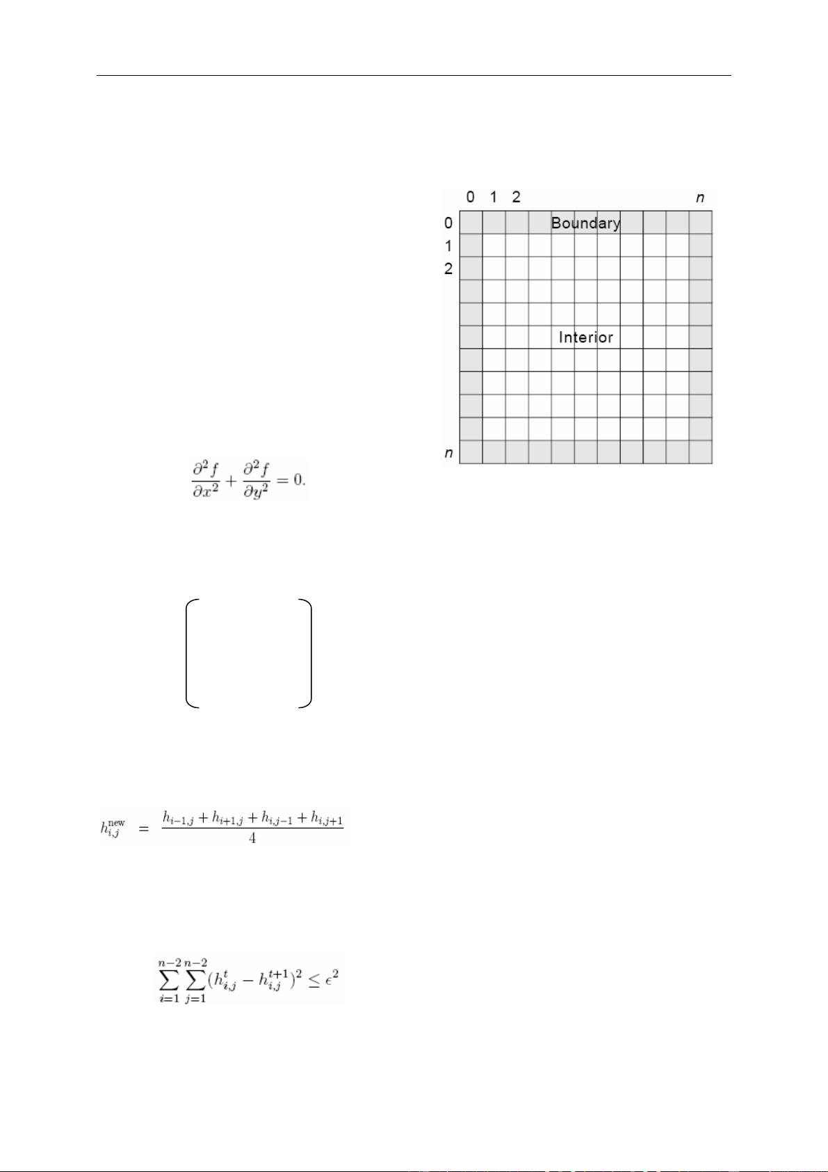
We can define the problem as a square metal plate is
divided into an (n+1) × (n+1) mesh of points (Figure
2.1).
Figure 2.1 Mesh with boundary and interior points
We update all the interior points using (1), leaving
the boundary points unchanged, and storing the new
values in a temporary mesh so as not to wipe out the
old values before we're done using them. Then we
replace the old values with the new values, and repeat
until a suitable termination criterion is achieved.
[5]
From section 2 to section 6 of this paper is the main
work we did in this problem. At the section 2 we
developed a sequential program to implement this
problem and we analyze the complexity of it. At the
section 3 we developed a parallel platform and used
parallel algorithm to implement the problem At the
section 4 we compare the sequential algorithm with
parallel algorithm by using the outputs. At the section
5 we analyzed the parallel algorithm’s complexity
and showed how our theoretical analysis compares to
practical results. At the section 6 we provided a chart
that shows a prediction of the speedup as we use
more processors.
2. Sequential algorithm and complexity:
The sequential implementation of this problem is as
follows:
First of all, we should initialize an n×n matrix H
which stores the initial values of the boundary points
and internal points. The pseudo-code is as follows:

3
for(i=0;i<n;i++)
for(j=0;j<n;j++)
h[i][j] = initialvalue;
for(i=1;i<n-1;i++)
for(j=1;j<n-1;j++)
h[i][j]=0;
Then we start to update every element and store them
into a temporary matrix tmp[i][j], meanwhile
compute the variance. If the variance is less than ε the
computation will stop. The main pseudo-code is as
follows:
while(true)
{
for(i=1;i<n-1;i++)
for(j=1;j<n-1;j++)
hnew[i][j]=0.25*(h[i-1][j]+h[i+1][j]+h[i][j-
1]+[i][j+1]);
tmp[i][j]=hnew[i][j];
if(Variance < ε
2
)break;
}
Sequential Complexity:
From the code above we can see that the each step
the computation of Jacobi’s iterations runs n×n times.
Because the first loop is from 1 to n-1 (0 and n is the
boundary), when the first loop finish the second loop
will begin from 1 to n-1(0 and n is the boundary). So
the complexity is
T=O(n×n)=O(n²).
3 Parallel mechanisms
In this section, we will expound our platform and
algorithm used in this project for parallelizing heat
distributing problem, and ultimately implementing
two versions of parallel algorithms based on blocking
and nonblocking communication respectively.
3.1 Parallel platform
In this project, we implement our parallel algorithm
by MPI which is a standardized API typically used
for parallel and/or distributed computing
[1]
. Further
more, we compile and run our jobs with Open MPI.
Before discuss functions used in our programs, we
learn some basic concepts of MPI.
MPI is not a revolutionary new way of programming
parallel computers. Rather, it is an attempt to collect
the best features of many message-passing systems
that have been developed over the years, improve
them where appropriate, and standardize them
[3]
.
MPI is a library, not a language.
MPI is a specification, not a particular
implementation.
MPI address the message-passing model.
MPI programs consist of processes that are
automatically distributed over a set of machines, each
process being given a unique identifier called a rank.
MPI processes are not spawned as required, but
rather all processes are determined at the command
line when starting the MPI application
[4]
.
In the message-passing model of parallel computation,
the processes executing in parallel have separate
address spaces. Communication occurs when a
portion of one process’s address space is copied into
another process’s address space. This operations is
cooperative and occurs only when the first process
executes a send operations and the second process
executes a receive operation.
In our blocking communication version (heatParaB.c),
we use the MPI_Sendrecv() function to send and
receive message to/from other processes. The
send-receive operations combine in one call the
sending of a message to one destination and the
receiving of another message, from another process.
This send-receive operation is very useful for
preventing cyclic dependencies that may lead to
deadlock
[2]
. When a send-receive operation is used,
the communication subsystem takes care of this issue.
One can improve performance on many systems by
overlapping communication and computation.
Nonblocking communication is an alternative
mechanism that often leads to better performance
[2]
.
A nonblocking send start call initiates the send
operation, but does not complete it. The send start
call can return before the message was copied out of
the send buffer. With suitable hardware, the transfer
of data out of the sender memory may proceed
concurrently with computations done at the sender
after the send was initiated and before it completed.
Similarly, a nonblocking receive start call initiates the
receive operation, but does not complete it. The call
can return before a message is stored into the receive


- 1
- 2
前往页