没有合适的资源?快使用搜索试试~ 我知道了~
资源推荐
资源详情
资源评论
4
Chapter
Mobile Robot Vehicles
helpful to consider some general, but important, concepts regarding mobility.
4.1
l
Mobility
We have already touched on the diversity of mobile robots and their modes of locomo-
tion. In this section we will discuss mobility which is concerned with how a vehicle
moves in space.
We first consider the simple example of a train. The train moves along rails and its posi-
tion is described by its distance along the rail from some datum. The configuration of the
train can be completely described by a scalar parameter q which is called its generalized
coordinate. The set of all possible configurations is the configuration space, or C-space, de-
noted by C and q∈C. In this case C ⊂R. We also say that the train has one degree of free-
dom since q is a scalar. The train also has one actuator (motor) that propels it forwards or
backwards along the rail. With one motor and one degree of freedom the train is fully
actuated and can achieve any desired configuration, that is, any position along the rail.
Another important concept is task space which is the set of all possible poses ξ of
the vehicle and ξ ∈ T. The task space depends on the application or task. If our task
was motion along the rail then T ⊂ R. If we cared only about the position of the train
in a plane then T ⊂ R
2
. If we considered a 3-dimensional world then T ⊂ SE(3), and its
height changes as it moves up and down hills and its orientation changes as it moves
around curves. Clearly for these last two cases the dimensions of the task space exceed
the dimensions of the configuration space and the train cannot attain an arbitrary
pose since it is constrained to move along fixed rails. In these cases we say that the
train moves along a manifold in the task space and there is a mapping from q ξ.
Interestingly many vehicles share certain characteristics with trains – they are good
at moving forward but not so good at moving sideways. Cars, hovercrafts, ships and
aircraft all exhibit this characteristic and require complex manoeuvring in order to
move sideways. Nevertheless this is a very sensible design approach since it caters to
the motion we most commonly require of the vehicle. The less common motions such
as parking a car, docking a ship or landing an aircraft are more complex, but not im-
possible, and humans can learn this skill. The benefit of this type of design comes
from simplification and in particular reducing the number of actuators required.
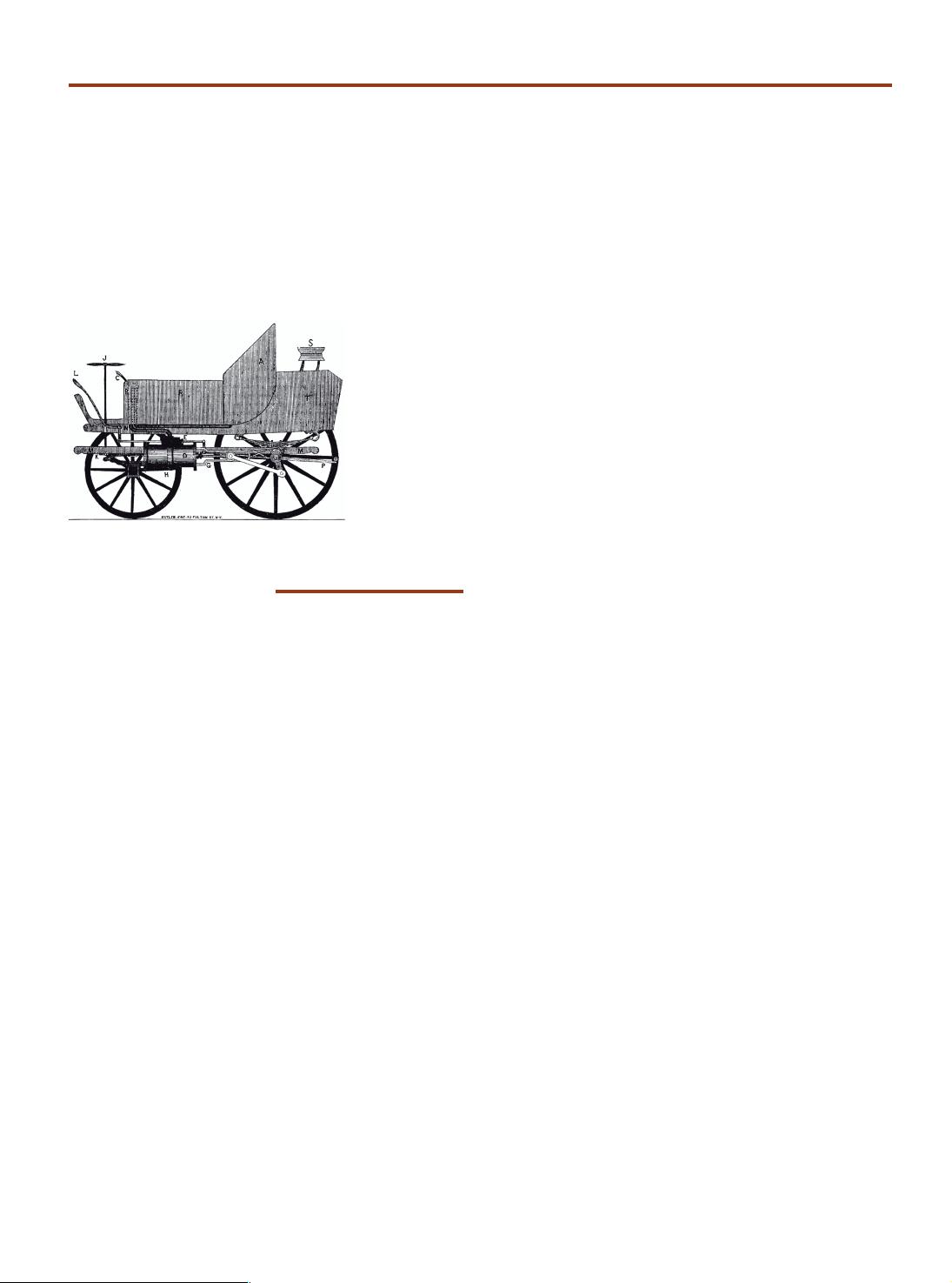
This chapter discusses how a robot platform moves, that is, how its pose
changes with time as a function of its control inputs. There are many differ-
ent types of robot platform as shown on pages 61–63 but in this chapter we
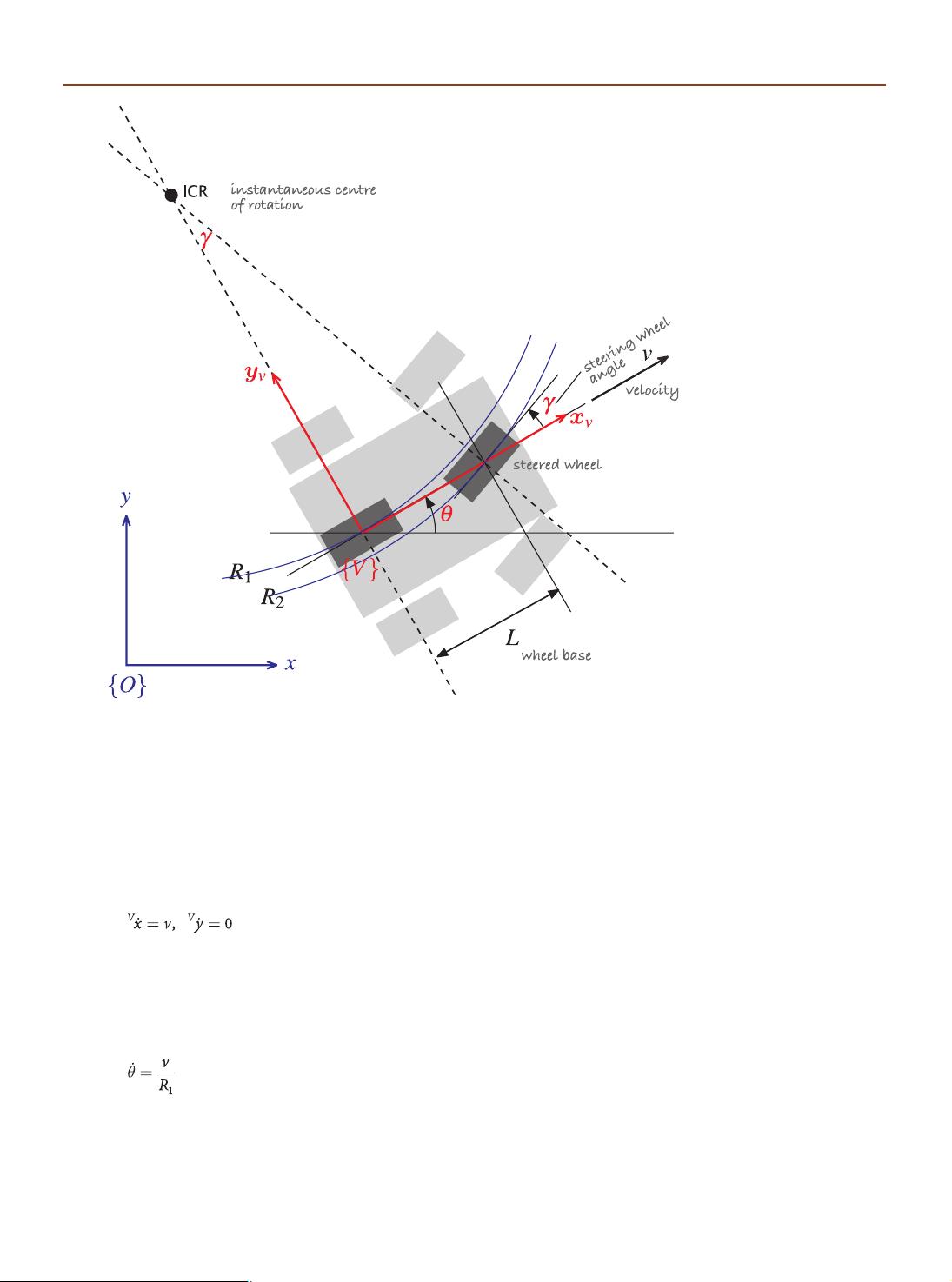
will consider only two which are important exemplars. The first is a wheeled
vehicle like a car which operates in a 2-dimensional world. It can be pro-
pelled forwards or backwards and its heading direction controlled by chang-
ing the angle of its steered wheels. The second platform is a quadcopter, a
flying vehicle, which is an example of a robot that moves in 3-dimensional
space. Quadcopters are becoming increasing popular as a robot platform
since they can be quite easily modelled and controlled.
However before we start to discuss these two robot platforms it will be
66
Next consider a hovercraft which has two propellors whose axes are parallel but not
collinear. The sum of their thrusts provide a forward force and the difference in thrusts
generates a yawing torque for steering. The hovercraft moves over a planar surface
and its configuration is entirely described by three generalized coordinates
q = (x, y, θ) ∈ C and in this case C ⊂ R
2
× S. The configuration space has 3 dimen-
sions and the vehicle therefore has three degrees of freedom.
The hovercraft has only two actuators, one fewer than it has degrees of freedom,
and it is therefore an under-actuated system. This imposes limitations on the way in
which it can move. At any point in time we can control the forward (parallel to the
thrust vectors) acceleration and the rotational acceleration of the the hovercraft but
there is zero sideways (or lateral) acceleration since it does not generate any lateral
thrust. Nevertheless with some clever manoeuvring, like with a car, the hovercraft can
follow a path that will take it to a place to one side of where it started. The advantage of
under-actuation is the reduced number of actuators, in this case two instead of three.
The penalty is that the vehicle cannot move directly to an any point in its configura-
tion space, it must follow some path. If we added a third propellor to the hovercraft
with its axis normal to the first two then it would be possible to command an arbitrary
forward, sideways and rotational acceleration. The task space of the hovercraft is
T ⊂ SE(2) which is equivalent, in this case, to the configuration space.
A helicopter has four actuators. The main rotor generates a thrust vector whose
magnitude is controlled by the collective pitch, and the thrust vector’s direction is
controlled by the lateral and longitudinal cyclic pitch. The fourth actuator, the tail
rotor, provides a yawing moment. The helicopter’s configuration can be described by
six generalized coordinates q = (x, y, z, θ
r
, θ
p
, θ
y
) ∈ C which is its position and orienta-
tion in 3-dimensional space, with orientation expressed in roll-pitch-yaw angles. The
configuration space C ⊂ R
3
× S
3
has six dimensions and therefore the vehicle has six
degrees of freedom. The helicopter is under-actuated and it has no means to rotationally
accelerate in the pitch and roll directions but cleverly these unactuated degrees of
freedom are not required for helicopter operation – the helicopter naturally maintains
stable equilibrium values for roll and pitch angle. Gravity acts like an additional actua-
tor and provides a constant downward force. This allows the helicopter to accelerate
sideways using the horizontal component of its thrust vector, while the vertical com-
ponent of thrust is counteracted by gravity – without gravity a helicopter could not fly
sideways. The task space of the helicopter is T ⊂ SE(3).
A fixed-wing aircraft moves forward very efficiently and also has four actuators
(forward thrust, ailerons, elevator and rudder). The aircraft’s thrust provides accelera-
tion in the forward direction and the control surfaces exert various moments on the
aircraft: rudder (yaw torque), ailerons (roll torque), elevator (pitch torque). The aircraft’s
configuration space is the same as the helicopter and has six dimensions. The aircraft
is under-actuated and it has no way to accelerate in the lateral direction. The task
space of the aircraft is T ⊂ SE(3).
The DEPTHX underwater robot shown on page 62 also has a configuration space
C ⊂ R
3
× S
3
of six dimensions, but by contrast is fully actuated. Its six actuators can
exert an arbitrary force and torque on the vehicle, allowing it to accelerate in any di-
rection or about any axis. Its task space is T ⊂ SE(3).
Finally we come to the wheel – one of humanity’s greatest achievements. The wheel
was invented around 3000 bce and the two wheeled cart was invented around 2000 bce.
Today four wheeled vehicles are ubiquitous and the total automobile population of the
planet is approaching one billion.
The effectiveness of cars, and our familiarity with
them, makes them a natural choice for robot platforms that move across the ground.
The configuration of a car moving over a plane is described by its generalized coor-
dinates q = (x, y, θ) ∈ C and C ⊂ R
2
× S which has 3 dimensions. A car has only two
actuators, one to move forwards or backwards and one to change the heading direc-
tion. The car is therefore under-actuated.
As we have already remarked an under-
actuated vehicle cannot move directly to an any point in its configuration space, it
Some low-cost hobby aircraft have no
rudder and rely only on ailerons to bank
and turn the aircraft. Even cheaper
hobby aircraft have no elevator and rely
on engine speed to control height.
http://hypertextbook.com/facts/2001/
MarinaStasenko.shtml.
Unlike the aircraft and underwater ro-
bot the motion of a car is generally con-
sidered in terms of velocities rather
than forces and torques.
Chapter 4
·
Mobile Robot Vehicles
67
must follow generally nonlinear some path. We know from our everyday experience
with cars that it is not possible to drive sideways, but with some practice we can learn
to follow a path that results in the vehicle being to one side of its initial position – this
is parallel parking. Neither can a car rotate on spot, but we can follow a path that
results in the vehicle being at the same position but rotated by 180° – a three-point
turn. The challenges this introduces for control and path planning will be discussed in
the rest of this part of the book. Despite this limitation the car is the simplest and most
effective means of moving in a planar world that we have yet found.
The standard wheel is highly directional and prefers to roll in the direction normal
to the axis of rotation. We might often wish for an ability to roll sideways but the stan-
dard wheel provides significant benefit when cornering – lateral friction between the
wheels and the road counteracts, for free, the centripetal acceleration which would
otherwise require an extra actuator to provide that force. More radical types of wheels
have been developed that can roll sideways. An omni-directional wheel or Swedish
wheel is shown in Fig. 4.1. It is similar to a normal wheel but has a number of passive
rollers around its circumference and their rotational axes lie in the plane of the wheel.
It is driven like an ordinary wheel but has very low friction in the lateral direction. A
spherical wheel is similar to the roller ball in an old-fashioned computer mouse but
driven by two actuators so that it can achieve achieve a velocity in any direction.
In robotics a car is often described as a non-holonomic vehicle. The term non-
holonomic comes from mathematics and means that the motion of the car is subject
to one or more non-holonomic constraints. A holonomic constraint is an equation
that can be written in terms of the configuration variables x, y and θ. A non-holonomic
constraint can only be written in terms of the derivatives of the configuration vari-
ables and cannot be integrated to a constraint in terms of configuration variables. Such
systems are therefore also known as non-integrable systems. A key characteristic of
these systems, as we have already discussed, is that they cannot move directly from one
configuration to another – they must perform a manoeuvre or sequence of motions
.
A skid-steered vehicle, such as a tank, can turn on the spot but to move sideways it
would have to stop, turn, proceed, stop then turn – this is a manoeuvre or time-vary-
ing control strategy which is the hallmark of a non-holonomic system. The tank has
two actuators, one for each track, and just like a car is under-actuated.
Mobility parameters for the vehicles that we have discussed are tabulated in Table 4.1.
The second column is the number of degrees of freedom of the vehicle or the dimen-
sion of its configuration space. The third column is the number of actuators and the
fourth column indicates whether or not the vehicle is fully actuated.
4.2
l
Car-like Mobile Robots
Wheeled cars are a very effective class of vehicle and the archetype for most ground
robots such as those shown on page 62. In this section we will create a model for a car-
like vehicle and develop controllers that can drive the car to a point, along a line, follow
an arbitrary path, and finally, drive to a specific pose.
Fig. 4.1. Omni-directional (or
Swedish) wheel. Note the circum-
ferential rollers which make mo-
tion in the direction of the wheel’s
axis almost frictionless. (Courtesy
Vex Robotics)
Table 4.1.
Summary of parameters for
three different types of vehicle.
The +g notation indicates that
the gravity field can be consid-
ered as an extra actuator
We can also consider this in control theo-
retic terms. Brockett’s theorem (Brockett
1983) states that such systems are con-
trollable but they cannot be stabilized
to a desired state using a differentiable,
or even continuous, pure state feedback
controller. A time varying or non-linear
control strategy is required.
4.2 · Car-like Mobile Robots
68
A commonly used model for a four-wheeled car-like vehicle is the bicycle model
shown in Fig. 15.1. The bicycle has a rear wheel fixed to the body and the plane of the
front wheel rotates about the vertical axis to steer the vehicle.
The pose of the vehicle is represented by the coordinate frame {V} shown in Fig. 4.2,
with its x-axis in the vehicle’s forward direction and its origin at the centre of the rear
axle. The configuration of the vehicle is represented by the generalized coordinates
q = (x, y, θ) ∈ C where C ⊂ SE(2). The vehicle’s velocity
is by definition v in the vehicle’s
x-direction, and zero in the y-direction since the wheels cannot slip sideways. In the
vehicle frame {V} this is
The dashed lines show the direction along which the wheels cannot move, the lines
of no motion, and these intersect at a point known as the Instantaneous Centre of
Rotation (ICR). The reference point of the vehicle thus follows a circular path and its
angular velocity is
(4.1)
and by simple geometry the turning radius is R
1
= L /tanγ where L is the length of
the vehicle or wheel base. As we would expect the turning circle increases with vehicle
length. The steering angle γ is limited mechanically and its maximum value dictates
the minimum value of R
1
.
Fig. 4.2.
Bicycle model of a car. The car
is shown in light grey, and the
bicycle approximation is dark
grey. The vehicle’s coordinate
frame is shown in red, and the
world coordinate frame in blue.
The steering wheel angle is γ
and the velocity of the back
wheel, in the x-direction, is v. The
two wheel axes are extended as
dashed lines and intersect at the
Instantaneous Centre of Rotation
(ICR) and the distance from the
ICR to the back and front wheels
is R
1
and R
2
respectively
Often incorrectly called the Ackerman
model.
Other well known models include the
Reeds-Shepp model which has only
three speeds: forward, backward and
stopped, and the Dubbins car which has
only two speeds: forward and stopped.
Chapter 4
·
Mobile Robot Vehicles
69
For a fixed steering wheel angle the car moves along a circular arc. For this reason
curves on roads are circular arcs or clothoids
which makes life easier for the driver since
constant or smoothly varying steering wheel angle allow the car to follow the road. Note
that R
2
> R
1
which means the front wheel must follow a longer path and therefore rotate
more quickly than the back wheel. When a four-wheeled vehicle goes around a corner the
two steered wheels follow circular paths of different radius and therefore the angles of the
steered wheels γ
L
and γ
R
should be very slightly different. This is achieved by the com-
monly used Ackerman steering mechanism which results in lower wear and tear on the
tyres. The driven wheels must rotate at different speeds on corners which is why a differ-
ential gearbox is required between the motor and the driven wheels.
The velocity of the robot in the world frame is (v cosθ, vsinθ) and combined with
Eq. 4.1 we write the equations of motion as
(4.2)
This model is referred to as a kinematic model since it describes the velocities of the vehi-
cle but not the forces or torques that cause the velocity. The rate of change of heading Ë is
referred to as turn rate, heading rate or yaw rate and can be measured by a gyroscope. It can
also be deduced from the angular velocity of the wheels on the left- and right-hand sides
of the vehicle which follow arcs of different radius and therefore rotate at different speeds.
In the world coordinate frame we can write an expression for velocity in the vehicle’s
y-direction
which is the non-holonomic constraint. This equation cannot be integrated to form a
relationship between x, y and θ.
Equation 4.2 captures some other important characteristics of a wheeled vehicle.
When v = 0 then Ë = 0, that is, it is not possible to change the vehicle’s orientation
when it is not moving. As we know from driving we must be moving in order to turn.
If the steering angle is ü then the front wheel is orthogonal to the back wheel, the
vehicle cannot move forward and the model enters an undefined region.
Vehicle coordinate system. The coordinate system that we will use, and a common one for vehicles
of all sorts is that the x-axis is forward (longitudinal motion), the y-axis is to the left side (lateral
motion) which implies that the z-axis is upward. For aerospace and underwater applications the
z-axis is often downward and the x-axis is forward.
Paths that arcs with smoothly varying
radius.
Rudolph Ackerman (1764–1834) was a German inventor born at Schneeberg, in Saxony. For finan-
cial reasons he was unable to attend university and became a saddler like his father. For a time he
worked as a saddler and coach-builder and in 1795 established a print-shop and drawing-school in
London. He published a popular magazine “The Repository of Arts, Literature, Commerce, Manu-
factures, Fashion and Politics” that included an eclectic mix of articles on water pumps, gas-light-
ing, and lithographic presses, along with fashion plates and furniture designs. He manufactured
paper for landscape and miniature painters, patented a method for waterproofing cloth and paper
and built a factory in Chelsea to produce it. He is buried in Kensal Green Cemetery, London.
In 1818 Ackermann took out British patent 4212 on behalf of the German inventor George
Lankensperger for a steering mechanism which ensures that the steered wheels move on circles
with a common centre. The same scheme was proposed and tested by Erasmus Darwin (grandfa-
ther of Charles) in the 1760s. Subsequent refinement by the Frenchman Charles Jeantaud led to
the mechanism used in cars to this day which is known as Ackermann steering.
4.2 · Car-like Mobile Robots
剩余21页未读,继续阅读
资源评论
qq_14903801
- 粉丝: 5
- 资源: 25
上传资源 快速赚钱
- 我的内容管理 展开
- 我的资源 快来上传第一个资源
- 我的收益 登录查看自己的收益
- 我的积分 登录查看自己的积分
- 我的C币 登录后查看C币余额
- 我的收藏
- 我的下载
- 下载帮助
安全验证
文档复制为VIP权益,开通VIP直接复制
信息提交成功