1
Two-Dimensional Phase Unwrapping Problem
By Dr. Munther Gdeisat and Dr. Francis Lilley
Pre-requisite: In order to understand this tutorial it is necessary for you to have already studied and
completed the “one-dimensional phase unwrapping problem” tutorial before reading this document.
There are many applications that produce wrapped phase images. Examples of these are synthetic aperture
radar (SAR), magnetic resonance imaging (MRI) and fringe pattern analysis. The wrapped phase images that
are produced by these applications are not usable unless they are first unwrapped so as to form a
continuous phase map. This means that the development of a robust phase unwrapping algorithm is an
important topic for all these applications. In this article, we will not discuss phase unwrapping only in the
specific context of these applications, but we will instead explain the concept of the 2D phase unwrapping
problem in general terms.
1. Introduction to 2D phase unwrapping
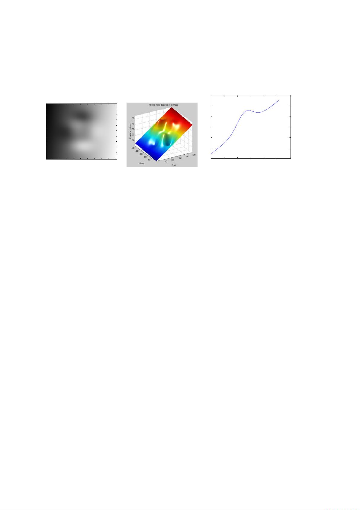
We shall explain the 2D phase unwrapping process as follows. Suppose that we have a computer-generated
continuous phase image that does not contain any phase wraps (2π jumps). This image may be displayed as
a visual intensity array, as shown in Figure 1(a). The same image may also be plotted as a 3D surface, as
shown in Figure 1(b). The intensities from a single row of this image (row 410) are graphically plotted in
Figure 1(c). The Matlab code that is used to generate this phase image is as follows. The peaks Matlab
function is used to generate the continuous phase image. Please note that we are using the term
“continuous” here to refer not to an analogue signal, but to a discrete 1D phase signal, or a discrete 2D
phase image, that does not contain any phase wraps.
%This program is to simulate a continuous phase distribution to act as a dataset
%for use in the 2D phase unwrapping problem
clc; close all; clear
N = 512;
[x,y]=meshgrid(1:N);
image1 = 2*peaks(N) + 0.1*x + 0.01*y;
figure, colormap(gray(256)), imagesc(image1)
title('Continuous phase image displayed as a visual intensity array')
xlabel('Pixels'), ylabel('Pixels')
figure
surf(image1,'FaceColor','interp', 'EdgeColor','none', 'FaceLighting','phong')
view(-30,30), camlight left, axis tight
title(' Continuous phase map image displayed as a surface plot')
xlabel('Pixels'), ylabel('Pixels'), zlabel('Phase in radians')
figure, plot(image1(410,:))
title('Row 410 of the continuous phase image')
xlabel('Pixels'), ylabel('Phase in radians')