


CS231A Course Notes 4: Stereo Systems and
Structure from Motion
Kenji Hata and Silvio Savarese
1 Introduction
In the previous notes, we covered how adding additional viewpoints of a
scene can greatly enhance our knowledge of the said scene. We focused on
the epipolar geometry setup in order to relate points of one image plane to
points in the other without extracting any information about the 3D scene.
In these lecture notes, we will discuss how to recover information about the
3D scene from multiple 2D images.
2 Triangulation
One of the most fundamental problems in multiple view geometry is the
problem of triangulation, the process of determining the location of a 3D
point given its projections into two or more images.
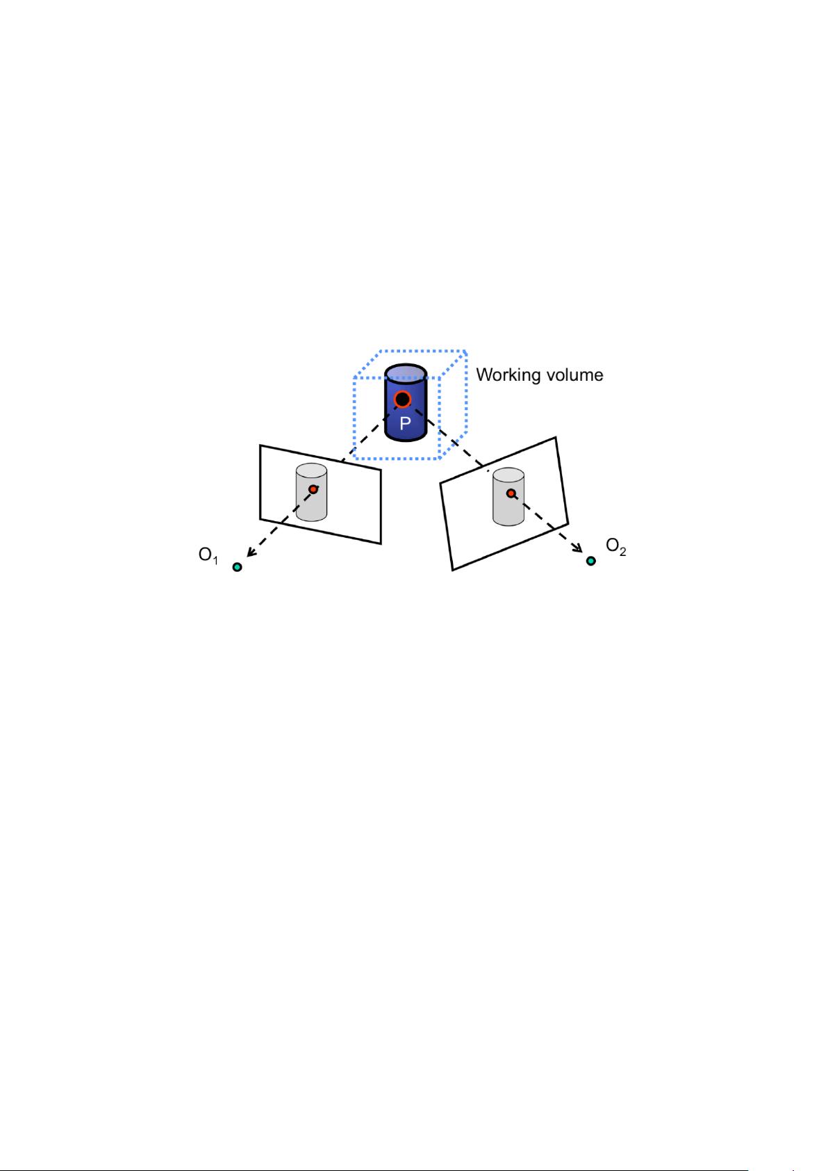
Figure 1: The setup of the triangulation problem when given two views.
1

In the triangulation problem with two views, we have two cameras with
known camera intrinsic parameters K and K
0
respectively. We also know the
relative orientations and offsets R, T of these cameras with respect to each
other. Suppose that we have a point P in 3D, which can be found in the
images of the two cameras at p and p
0
respectively. Although the location of
P is currently unknown, we can measure the exact locations of p and p
0
in
the image. Because K, K
0
, R, T are known, we can compute the two lines of
sight ` and `
0
, which are defined by the camera centers O
1
, O
2
and the image
locations p, p
0
. Therefore, P can be computed as the intersection of ` and `
0
.
Figure 2: The triangulation problem in real-world scenarios often involves
minimizing the reprojection error.
Although this process appears both straightforward and mathematically
sound, it does not work very well in practice. In the real world, because the
observations p and p
0
are noisy and the camera calibration parameters are
not precise, finding the intersection point of ` and `
0
may be problematic. In
most cases, it will not exist at all, as the two lines may never intersect.
2.1 A linear method for triangulation
In this section, we describe a simple linear triangulation method that solves
the lack of an intersection point between rays. We are given two points in the
images that correspond to each other p = MP = (x, y, 1) and p
0
= M
0
P =
(x
0
, y
0
, 1). By the definition of the cross product, p × (MP ) = 0. We can
2

explicitly use the equalities generated by the cross product to form three
constraints:
x(M
3
P ) −(M
1
P ) = 0
y(M
3
P ) − (M
2
P ) = 0
x(M
2
P ) − y(M
1
P ) = 0
(2.1)
where M
i
is the i-th row of the matrix M. Similar constraints can be for-
mulated for p
0
and M
0
. Using the constraints from both images, we can
formulate a linear equation of the form AP = 0 where
A =
xM
3
− M
1
yM
3
− M
2
x
0
M
0
3
− M
0
1
y
0
M
0
3
− M
0
2
(2.2)
This equation can be solved using SVD to find the best linear estimate of
the point P . Another interesting aspect of this method is that it can actu-
ally handle triangulating from multiple views as well. To do so, one simply
appends additional rows to A corresponding to the added constraints by the
new views.
This method, however is not suitable for projective reconstruction, as it is
not projective-invariant. For example, suppose we replace the camera matri-
ces M, M
0
with ones affected by a projective transformation MH
−1
, M
0
H
−1
.
The matrix of linear equations A then becomes AH
−1
. Therefore, a solution
P to the previous estimation of AP = 0 will correspond to a solution HP for
the transformed problem (AH
−1
)(HP ) = 0. Recall that SVD solves for the
constraint that kP k = 1, which is not invariant under a projective transfor-
mation H. Therefore, this method, although simple, is often not the optimal
solution to the triangulation problem. -
2.2 A nonlinear method for triangulation
Instead, the triangulation problem for real-world scenarios is often mathe-
matically characterized as solving a minimization problem:
min
ˆ
P
kM
ˆ
P − pk
2
+ kM
0
ˆ
P − p
0
k
2
(2.3)
In the above equation, we seek to find a
ˆ
P in 3D that best approximates P
by finding the best least-squares estimate of the reprojection error of
ˆ
P in
both images. The reprojection error for a 3D point in an image is the distance
between the projection of that point in the image and the corresponding
3
observed point in the image plane. In the case of our example in Figure 2,
since M is the projective transformation from 3D space to image 1, the
projected point of
ˆ
P in image 1 is M
ˆ
P . The matching observation of
ˆ
P
in image 1 is p. Thus, the reprojection error for image 1 is the distance
kM
ˆ
P − pk. The overall reprojection error found in Equation 2.3 is the sum
of the reprojection errors across all images. For cases with more than two
images, we would simply add more distance terms to the objective function:
min
ˆ
P
X
i
kM
ˆ
P
i
− p
i
k
2
(2.4)
In practice, there exists a variety of very sophisticated optimization tech-
niques that result in good approximations to the problem. However, for the
scope of the class, we will focus on only one of these techniques, which is the
Gauss-Newton algorithm for nonlinear least squares. The general nonlinear
least squares problem is to find an x ∈ R
n
that minimizes
kr(x)k
2
=
m
X
i=1
r
i
(x)
2
(2.5)
where r is any residual function r : R
n
→ R
m
such that r(x) = f(x) −
y for some function f, input x, and observation y. The nonlinear least
squares problem reduces to the regular, linear least squares problem when
the function f is linear. However, recall that, in general, our camera matrices
are not affine. Because the projection into the image plane often involves a
division by the homogeneous coordinate, the projection into the image is
generally nonlinear.
Notice that if we set e
i
to be a 2 × 1 vector e
i
= M
ˆ
P
i
− p
i
, then we can
reformulate our optimization problem to be:
min
ˆ
P
X
i
e
i
(
ˆ
P )
2
(2.6)
which can be perfectly represented as a nonlinear least squares problem.
In these notes, we will cover how we can use the popular Gauss-Newton
algorithm to find an approximate solution to this nonlinear least squares
problem. First, let us assume that we have a somewhat reasonable estimate
of the 3D point
ˆ
P , which we can compute by the previous linear method.
The key insight of the Gauss-Newton algorithm is to update our estimate by
correcting it towards an even better estimate that minimizes the reprojection
error. At each step we want to update our estimate
ˆ
P by some δ
P
:
ˆ
P =
ˆ
P + δ
P
.
4
But how do we choose the update parameter δ
P
? The key insight of the
Gauss-Newton algorithm is to linearize the residual function near the current
estimate
ˆ
P . In the case of our problem, this means that the residual error e
of a point P can be thought of as:
e(
ˆ
P + δ
P
) ≈ e(
ˆ
P ) +
∂e
∂P
δ
P
(2.7)
Subsequently, the minimization problem transforms into
min
δ
P
k
∂e
∂P
δ
P
− (−e(
ˆ
P ))k
2
(2.8)
When we formulate the residual like this, we can see that it takes the format
of the standard linear least squares problem. For the triangulation problem
with N images, the linear least squares solution is
δ
P
= −(J
T
J)
−1
J
T
e (2.9)
where
e =
e
1
.
.
.
e
N
=
p
1
− M
1
ˆ
P
.
.
.
p
n
− M
n
ˆ
P
(2.10)
and
J =
∂e
1
∂
ˆ
P
1
∂e
1
∂
ˆ
P
2
∂e
1
∂
ˆ
P
3
.
.
.
.
.
.
.
.
.
∂e
N
∂
ˆ
P
1
∂e
N
∂
ˆ
P
2
∂e
N
∂
ˆ
P
3
(2.11)
Recall that the residual error vector of a particular image e
i
is a 2 × 1
vector because there are two dimensions in the image plane. Consequently,
in the simplest two camera case (N = 2) of triangulation, this results in the
residual vector e being a 2N × 1 = 4 × 1 vector and the Jacobian J being a
2N ×3 = 4×3 matrix. Notice how this method handles multiple views seam-
lessly, as additional images are accounted for by adding the corresponding
rows to the e vector and J matrix. After computing the update δ
P
, we can
simply repeat the process for a fixed number of steps or until it numerically
converges. One important property of the Gauss-Newton algorithm is that
our assumption that the residual function is linear near our estimate gives
us no guarantee of convergence. Thus, it is always useful in practice to put
an upper bound on the number of updates made to the estimate.
5


